The syntax of growth() in lavaan is short and the models run in seconds. R returns fit statistics whether or not the time scores or the missing data make sense. Thus, we check these first. This chapter collects the checks that come before the first =~ line.
There is no growth model in this chapter. We use R (R Core Team, 2024), psych (Revelle, 2024), dplyr (Wickham et al., 2023), tidyr (Wickham et al., 2024) and ggplot2 (Wickham, 2016) to describe the data, and we use lavaan (Rosseel, 2012) for one small robustness run on the missing data. The models start in Chapter 2. Throughout the compendium we work with one dataset of 442 rows and 25 columns. Loneliness (lone1 to lone5), anxiety symptoms (anx1 to anx5), depression symptoms (dep1 to dep5) and hostility (host1 to host5) were measured at five waves, in 2015, 2016, 2018, 2019 and 2021. We use loneliness as the running example in this chapter. Every step applies in the same way to the other three variables.
1.1 Why look at the data first
The objectives of longitudinal research include describing change within persons and describing differences between persons in that change (Baltes & Nesselroade, 1979). A growth model addresses both objectives. The trajectory that it describes depends on the form and the time scores that you give it, and the foundational issues in modeling trajectories are discussed by McArdle (2012). If the form or the time scores are wrong, the model still returns numbers. For this reason, we look at the data before we model them.
The preliminary work answers four questions.
What does the average trajectory look like?
How stable is the relative standing of participants from one wave to the next?
How much information is missing, and where?
How are the waves spaced in time?
These questions can be answered with descriptive statistics, correlations, a missing data table and plots, and no latent variable is needed.
1.2 Descriptive statistics for each wave
1.2.1 The idea in plain language
Before we ask whether individuals change, we ask what the sample looks like at each wave. Flat sample means speak against a strong linear trend. Means that rise or fall steadily suggest that a straight line is a reasonable starting point. Means that rise and then fall suggest that one constant rate of change may not be enough. We also look at the shape of the distributions, because the estimation method in the workshop assumes multivariate normality.
1.2.2 R implementation
The function describe() from psych returns the number of observed values, the mean, the standard deviation and the shape of the distribution for each wave in one call.
Code
# Number of observed values, mean, standard deviation and shape of the distribution for each wavedesc_lone <-describe(data[, lone])desc_lone
# Addition: paired test of the change from the first to the third wave, complete casestt13 <-t.test(data$lone3[cc_lone], data$lone1[cc_lone], paired =TRUE)c(mean_diff =unname(tt13$estimate), t =unname(tt13$statistic), p = tt13$p.value)
  mean_diff           t           p
0.080062305 2.889456350 0.004122484
1.2.3 Understanding the output
The number of observed values differs between the waves. The scores are observed for 398, 395, 390, 413, 409 of the 442 participants at the five waves. This is the first sign of missing data, which the next section examines.
The means are 1.46, 1.47, 1.53, 1.35, 1.32 for 2015, 2016, 2018, 2019 and 2021. The mean is 0.07 higher in 2018 than in 2015, and it is lower in the last two waves. The mean in 2021 is 0.14 lower than the mean in 2015. The standard errors of the wave means are 0.023, 0.026, 0.026, 0.023, 0.019. The means for the 321 participants with complete data are given by the second chunk, and they show the same pattern. Among these participants the rise from 2015 to 2018 is 0.08 (paired t = 2.89, p = .004). It is small in size but distinguishable from zero, at about 2.9 standard errors. Thus, the average level is lower in 2021 than in 2015. The shape of the path is examined with the models.
The standard deviations are 0.46, 0.52, 0.52, 0.47, 0.39. The spread is smaller at the last wave. In a score with most values near the lowest observed value, a smaller spread can reflect a floor effect as much as a change in how much participants differ. For that reason we do not read the standard deviations as evidence about individual differences in change. The variances of the growth factors address this more directly.
The shape of the distributions matters as well. The lowest observed value is 1 at every wave and the medians are between 1.20 and 1.36. Thus, most participants score close to the bottom of the range and a few score much higher. The skewness is between 1.52 and 3.05 and the kurtosis is between 2.27 and 12.75. Across the 15 loneliness, anxiety and depression scores, the skewness ranges from 1.48 to 3.82.
Maximum likelihood, the default estimator in growth(), assumes that the observed variables are multivariate normal. With distributions as skewed as these, this assumption is doubtful. In a simulation study of confirmatory factor analysis, the maximum likelihood chi-square was inflated when the data were non-normal (Curran et al., 1996). That study does not cover growth models, so we take it as a reason for caution and not as a measure of the bias here. Standard errors can be affected as well. The robust version of maximum likelihood, called MLR in lavaan, gives standard errors and a scaled chi-square statistic that account for non-normality (Yuan & Bentler, 2000). We use it for one check in the section on missing data. The fit indices in the later chapters should be read with this caution in mind.
1.3 Correlations across waves
1.3.1 The idea in plain language
The wave means describe the sample as a whole. The correlations between waves describe the relative standing of participants. A participant who is comparatively high at one wave can stay comparatively high at later waves, or the ordering of participants can change. The means and the ordering of participants can change independently. A growth model represents both aspects. The means of the growth factors describe the average trajectory, and the variances of the growth factors describe how much participants differ in their starting point and their rate of change.
If a score were a stable characteristic with a little random noise, all pairs of waves would correlate about equally, whatever the distance between them. If the correlations become smaller as the time between the waves increases, relative standing may be changing gradually, and that would leave room for individual differences in change. The variance of a slope factor captures such differences. An autoregressive process or wave-specific variance can produce the same pattern, so the correlations alone do not settle the matter.
1.3.2 R implementation
Code
round(cor(data[, lone], use ="pairwise.complete.obs"), 2)
The following chunk is an addition to the workshop. It lists the same correlations next to the number of years between the two waves, because the waves are not equally spaced.
Code
# Addition: correlations ordered by the distance in years between the two wavesr_lone <-cor(data[, lone], use ="pairwise.complete.obs")years <-c(0, 1, 3, 4, 6)idx <-which(upper.tri(r_lone), arr.ind =TRUE)gap_tab <-data.frame(pair =paste(lone[idx[, 1]], lone[idx[, 2]], sep =" - "),years_apart =abs(years[idx[, 1]] - years[idx[, 2]]),r =round(r_lone[idx], 2))gap_tab[order(gap_tab$years_apart, -gap_tab$r), ]
The correlations are positive in every pair and they lie between 0.30 and 0.62. The pairs that are one year apart (lone1 and lone2, lone3 and lone4) correlate at 0.62 and 0.49. The two pairs that are two years apart correlate at 0.52 and 0.43, and the pair that is six years apart (lone1 and lone5) correlates at 0.30, which is the lowest value in the matrix. Notice that adjacent waves are not equally far apart. The correlations decrease with the years between the waves, although not perfectly. The pair lone3 and lone4 is one year apart and correlates at 0.49, which is lower than the pair lone2 and lone3 at two years apart (0.52).
The correlations are computed on all pairs of available values, so they rest on different numbers of participants. They are not the same as the correlations among the 321 complete cases that the models use.
1.3.4 Interpretation
The pattern is consistent with moderate stability of relative standing that fades slowly with time. No correlation is near zero, so participants who are comparatively high at the start tend to remain comparatively high. No correlation is near one. This is compatible with participants changing at different rates, but correlations that decrease with distance also arise from wave-specific variation or an autoregressive process, and a correlation matrix does not separate these from systematic change. A slope factor with some variance is therefore something to look for in Chapter 2, and the correlations do not establish it.
1.4 Missing data
1.4.1 How much is missing, and where
Every number above rests on whichever participants have data at that wave. Before we trust a model we need to know how much data is missing and in what pattern. This section is the one place in the compendium where listwise deletion, full information maximum likelihood (FIML) and the missing at random assumption are explained in full. The later chapters report the number of participants that each model used, give a short sensitivity result and refer to this section.
n_complete_lone <-sum(complete.cases(data[, lone]))n_complete_cov <-sum(complete.cases(data[, c("female", host)]))cat("Complete on all five loneliness waves:", n_complete_lone, "of", nrow(data), "\n")
Complete on all five loneliness waves: 321 of 442
Code
cat("Complete on female and all five hostility waves:", n_complete_cov, "of", nrow(data), "\n")
Complete on female and all five hostility waves: 320 of 442
Code
# Number of waves with an observed loneliness score, per participantn_waves <-rowSums(!is.na(data[, lone]))table(n_waves)
n_waves
  0   1   2   3   4   5
  6   6   8  26  75 321
Code
# Is a participant missing the same waves on all four measures?same_rows <-all(sapply(1:5, function(w) { m <-is.na(data[[paste0("lone", w)]])all(m ==is.na(data[[paste0("anx", w)]]) & m ==is.na(data[[paste0("dep", w)]]) & m ==is.na(data[[paste0("host", w)]]))}))same_rows
[1] TRUE
Code
# Participants with a missing wave that is followed by an observed waven_gap <-sum(apply(!is.na(data[, lone]), 1, function(o) any(!o[-5] &sapply(1:4, function(k) any(o[(k +1):5])))))n_gap
[1] 96
The number of missing values on the loneliness scores is 44, 47, 52, 29, 33 at the five waves. At every wave, the same participants are missing on all four repeated measures, which is why the counts for anx, dep and host repeat those of lone. Of the 442 rows, 321 have data at all five waves on loneliness (72.6 percent), and 320 have complete data on female and the five hostility scores. Further, 6 participants have no loneliness data at any wave. The variable female is missing for 27 participants, and the substance use score subs5, measured only at the last wave, is missing for 60 participants (13.6 percent), which is the largest count of any variable. The variables pdu1 and ace1 are missing for 27 participants each. They are not used in the models of this compendium.
The table of the number of observed waves shows that most participants with missing values still have data at several waves. The missing values are also not only the result of participants leaving the study. For 96 participants a missing wave is followed by a later wave with data. Several mechanisms can produce such patterns, and the dataset does not tell us which one operated.
1.4.2 What the workshop script does
The workshop script calls growth() with its default settings. The default for missing data in lavaan is listwise deletion, so a participant who is missing on any of the variables in the model is removed before estimation. For the loneliness models this leaves 321 of 442 participants, and lavaan reports it in the line “Used” and “Total” in the summary. The models that include covariates or an outcome measured once use fewer participants, and the multigroup models also drop the participants with missing female. In that case lavaan prints the message that the group variable contains missing values. Take the number of participants that a model used from the lavaan output and not from the number of rows in the dataset.
Listwise deletion is simple to apply and to report. It costs power, because 121 participants (27.4 percent of the rows) contribute nothing, even though most of them have data at some waves. It can also bias the estimates, if the participants who are dropped differ from those who are kept in ways that are related to the scores (Enders, 2010).
1.4.3 Listwise deletion and full information maximum likelihood
Full information maximum likelihood (FIML) uses every available value. A participant with three observed waves contributes the information of those three waves to the likelihood. In lavaan, FIML is requested with missing = "fiml". Data are missing completely at random when the probability of a missing value is unrelated to any score, observed or not. They are missing at random (MAR) when this probability depends on observed values only, and missing not at random when it depends on the missing value itself, given the observed ones (Rubin, 1976). FIML gives valid estimates under MAR and under missing completely at random. Listwise deletion is valid only under the latter. In the simulation conditions that Enders & Bandalos (2001) examined, FIML was found to perform better than listwise deletion in structural equation models. Enders (2010) gives a full treatment. FIML as implemented in lavaan also assumes multivariate normality, so the caution about non-normality above applies to it as well.
Missing at random cannot be verified from the data, because the assumption concerns the values that we did not observe. We can only look for signs that the participants who are missing differ on what we do observe. The following chunk is an addition to the workshop. It compares the first loneliness score of the participants who have data at all five waves with that of the participants who have the first score but are missing at a later wave.
   n_incomplete mean_incomplete      n_complete   mean_complete               p
     77.0000000       1.5212987     321.0000000       1.4432606       0.2770001
The 77 participants who have a first score but are missing later have a mean of 1.52 at the first wave, against 1.44 for the 321 complete participants. The difference is small relative to its uncertainty (p = .28). This suggests that there is no large difference in initial level between the two groups. It does not show that the data are missing at random, since the later values of those who left are not observed, and a test with 77 participants has limited power.
Missing at random is an assumption
A table of missing values and a comparison of observed scores cannot prove that the missing values are missing at random. They can only show that nothing in the observed data contradicts it. Whether a method is justified depends on reasons for missingness that lie outside the data, so state the assumption when you report the method.
1.4.4 Sensitivity to the missing data handling
The workshop models are fitted with listwise deletion, and those are the numbers reported in the chapters. To see how much the handling of missing data matters, we fit the linear model of Chapter 2 twice, once with the default and once with FIML. The model syntax in the chunk below is the workshop syntax and has not been changed. The lines that request FIML, and everything that follows in this subsection, are an addition that was not part of the workshop.
Code
linear <-' i =~ 1*lone1 + 1*lone2 + 1*lone3 + 1*lone4 + 1*lone5 s =~ 0*lone1 + 1*lone2 + 3*lone3 + 4*lone4 + 6*lone5'fit_linear_lw <-growth(linear, data = data)# Addition (not in the workshop): the same model with FIMLfit_linear_fiml <-growth(linear, data = data, missing ="fiml")
The warning that lavaan prints for the FIML model says that some cases are empty and will be ignored. These are the participants without a single loneliness score. They cannot contribute to the likelihood of a model for these five variables, and there are 6 of them. With FIML the model uses 436 participants. With listwise deletion it uses 321.
# Addition: FIML with robust (MLR) standard errors and scaled test statisticfit_linear_mlr <-growth(linear, data = data, missing ="fiml", estimator ="MLR")round(fitMeasures(fit_linear_mlr, c("chisq.scaled", "df.scaled", "cfi.robust", "rmsea.robust")), 3)
The mean of the intercept factor is 1.466 with listwise deletion and 1.490 with FIML. The mean of the slope factor is -0.025 and -0.027. Hence, the estimated average starting level and the estimated average yearly change move little. The variances are somewhat larger with FIML. The intercept variance is 0.139 against 0.165, and the slope variance is 0.003 against 0.004. In both runs the covariance between the intercept and slope factors is negative, and the slope variance is small but above zero.
The fit looks better with FIML (CFI 0.892 against 0.852, RMSEA 0.118 against 0.143). The two fit statistics are not strictly comparable, because they come from different numbers of participants. Neither set reaches the combination rules that are commonly used for these indices (Hu & Bentler, 1999). The robust run gives a scaled chi-square of 38.77 on 10 degrees of freedom, against 70.82 for the standard FIML statistic, with CFI 0.902 and RMSEA 0.123. A smaller scaled statistic is in line with an inflated standard chi-square under non-normality, but the fit remains short of the usual benchmarks.
In short, the substantive reading of the linear model does not depend much on how the missing data are handled, but the variances and the fit statistics change more. The FIML result does not remove the uncertainty about the missing data mechanism. It rests on the same missing at random assumption that we cannot test.
1.5 Trajectory plots
1.5.1 The idea in plain language
Tables of means and correlations average over participants, and two quite different patterns of change can give the same means. Everyone can change in about the same way, or participants can differ a lot and cancel out on average. A plot with all participants shows the overall form and whether there are obvious clusters. A small set of individual panels shows what single trajectories look like.
1.5.2 R implementation
The scores are first rearranged from wide to long format, with one row per participant and wave.
Code
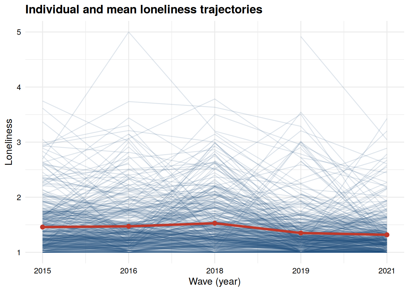
long_lone <- data %>%select(personid, lone1, lone2, lone3, lone4, lone5) %>%pivot_longer(cols =starts_with("lone"), names_to ="wave", values_to ="loneliness") %>%mutate(wave_num =as.numeric(gsub("lone", "", wave)),loneliness =suppressWarnings(as.numeric(loneliness)))ggplot(long_lone, aes(x = wave_num, y = loneliness, group = personid)) +geom_line(alpha =0.15, color ="#1f4e79") +stat_summary(aes(group =1), fun = mean, geom ="line", linewidth =1.4, color ="#c0392b") +stat_summary(aes(group =1), fun = mean, geom ="point", size =2.2, color ="#c0392b") +scale_x_continuous(breaks =1:5, labels =c("2015", "2016", "2018", "2019", "2021")) +labs(title ="Individual and mean loneliness trajectories",x ="Wave (year)", y ="Loneliness")
Figure 1.1: Individual loneliness trajectories (thin blue lines) with the sample mean trend overlaid (thick red line).
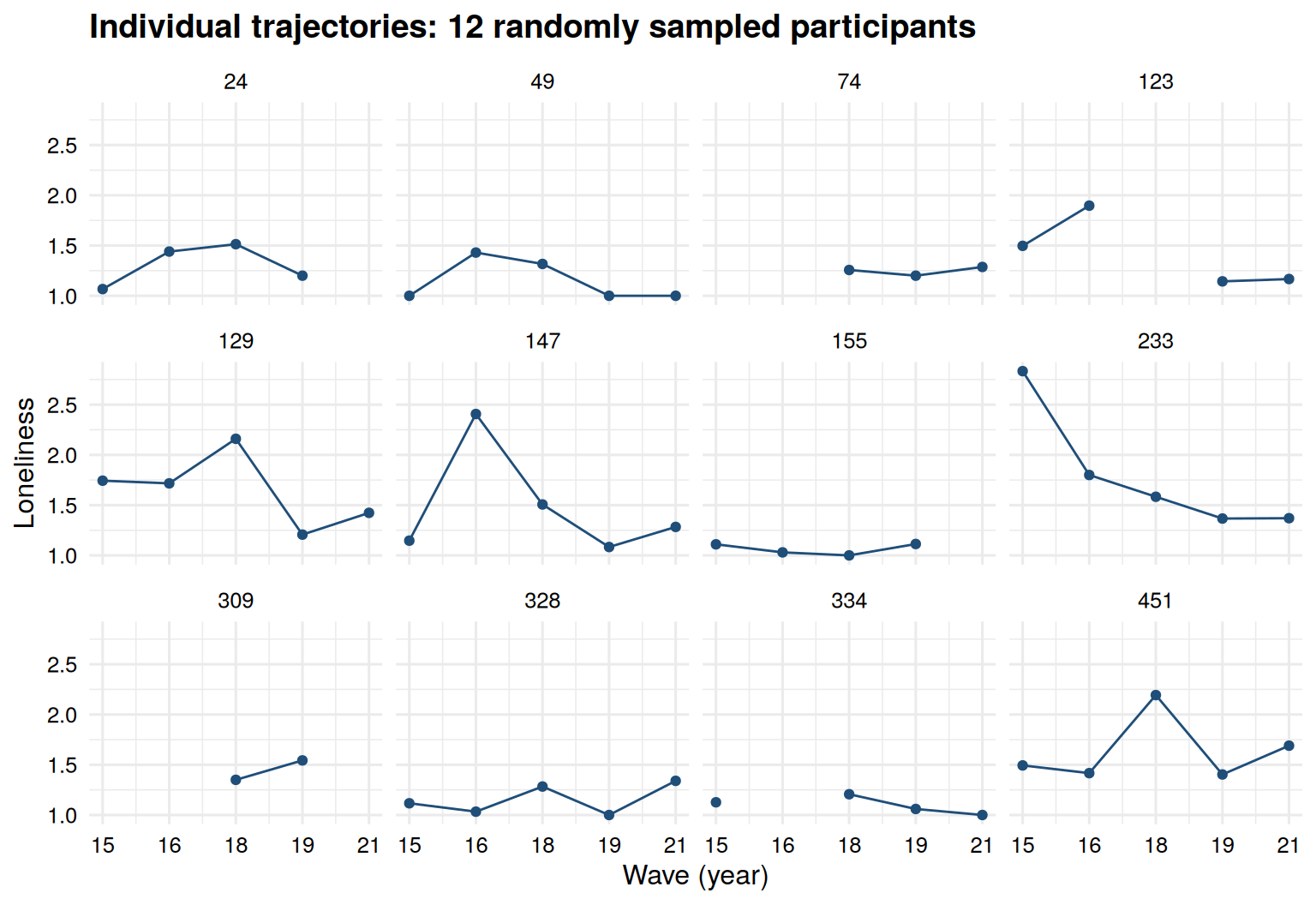
Figure 1.2: Individual trajectories for 12 randomly sampled participants.
Both plots place the five waves at equal distances on the horizontal axis, and the labels give the year. This is convenient for a first look, but it hides the unequal spacing of the waves. The next chunk is an addition to the workshop. It plots the wave means at their real position on the time axis. The vertical axis starts at 1, the lowest observed value, so that the differences between the means are not exaggerated.
Code
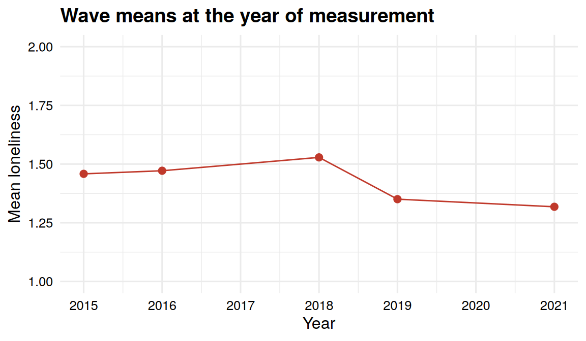
# Addition: wave means at the real calendar positionmean_tab <-data.frame(year =c(2015, 2016, 2018, 2019, 2021),mean_lone =colMeans(data[, lone], na.rm =TRUE))ggplot(mean_tab, aes(x = year, y = mean_lone)) +geom_line(color ="#c0392b") +geom_point(color ="#c0392b", size =2.2) +scale_x_continuous(breaks =2015:2021) +scale_y_continuous(limits =c(1, 2)) +labs(title ="Wave means at the year of measurement", x ="Year", y ="Mean loneliness")
Figure 1.3: Mean loneliness at each wave, placed at the year of measurement.
1.5.3 Understanding the output
Figure 1.1 shows a dense cloud of lines, and a mean line that follows the numbers in the descriptive table. A participant with a missing wave shows a gap in the line. The mean is computed from the observed values at each wave. The cloud does not separate into two obvious bundles, so there is no sign in this plot that the participants form clearly distinct groups. The lines are bunched near the bottom of the score range and a minority of participants reach much higher values, which agrees with the skewness reported earlier.
Figure 1.2 shows 12 participants, drawn at random with set.seed(42), each in a small panel. The panels differ from each other in level and in shape, and several contain gaps because of missing waves. Some participants stay close to the lowest values throughout, one participant peaks at the second wave and then falls, and one falls across the waves. Participants differ in where they start, and they also seem to differ in how their scores move over time. The statement that average loneliness is lower at the end does not describe any of these panels well. Twelve participants are a small sample, so these panels illustrate the variation and do not measure it. The growth models quantify it through the variances of the growth factors.
Figure 1.3 places the means on the calendar. The gaps between the waves alternate between one and two years. The distances on this axis are the ones that the time scores must represent.
1.6 Time scores
1.6.1 The idea in plain language
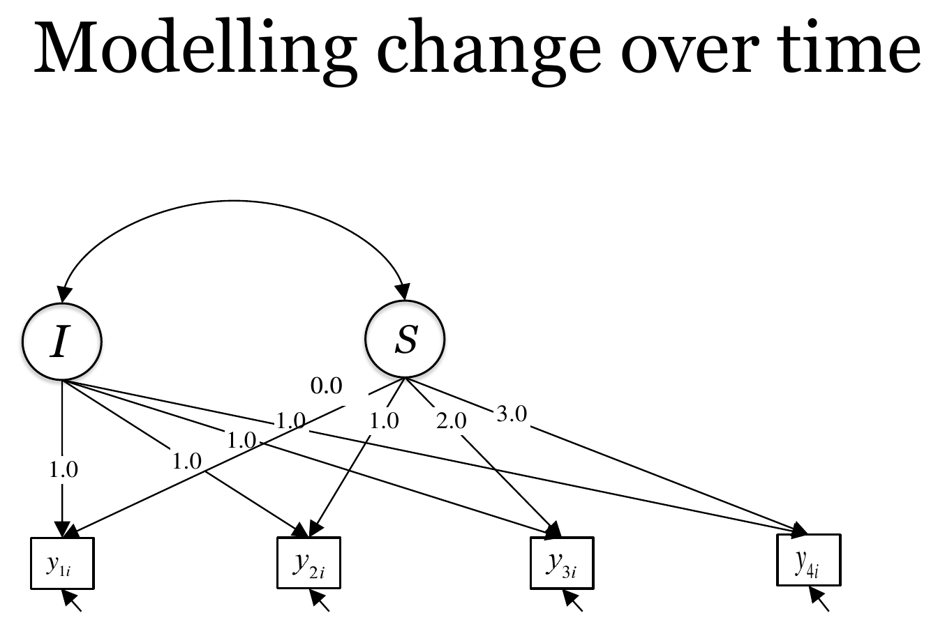
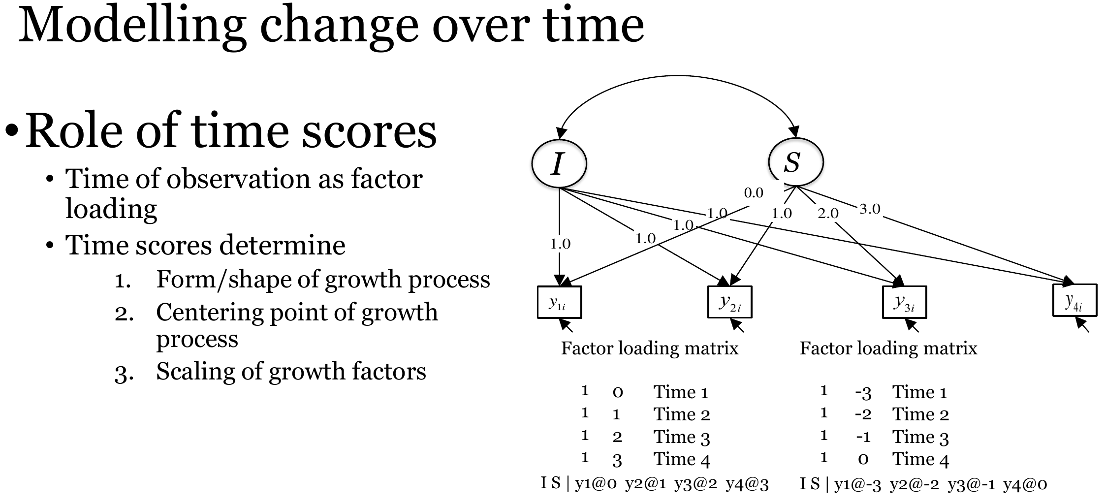
A growth model describes how the repeated measures change with time. The model needs to know when each measure was taken, and it receives this information through the loadings of the repeated measures on the slope factor. These loadings are the time scores. Figure 1.4 shows the basic model with an intercept factor I and a slope factor S and four repeated measures. The loadings of the measures on I are all 1, and the loadings on S are the time scores 0, 1, 2 and 3. The slide comes from the workshop, in which the models were estimated with Mplus and with R. It shows the structure of the model and no estimates. All numbers in this chapter come from the R output.
Figure 1.4: The basic growth model with an intercept factor (I) and a slope factor (S). The loadings on I are fixed to 1 and the loadings on S are the time scores. Look at the arrows from S to the measures, which carry the time scores. Source: workshop slides (Anyan, 2023).
The time scores set the form of the growth process, the centering point and the scaling of the growth factors, as Figure 1.5 lists. The right-hand side of the slide shows the same four waves coded in two ways. With the time scores 0, 1, 2 and 3 the intercept factor is the level at the first wave. With the time scores -3, -2, -1 and 0 the intercept factor is the level at the last wave. The slope has the same meaning in both, a change per unit of time, but the intercept and its variance describe a different moment.
Figure 1.5: The role of the time scores. Look at the two factor loading matrices on the right. They contain the same model with the intercept placed at the first wave (left matrix) and at the last wave (right matrix). Source: workshop slides (Anyan, 2023).
The pattern of the time scores sets the shape of the trajectory that the factors can represent. Time scores that increase in a straight line give a linear form. The quadratic model in Chapter 2 uses a third factor whose loadings are the squares of the time scores. The models in Chapter 3 use different time scores for different periods.
The time score of 0 marks the point where the intercept factor is defined. The mean of the intercept factor is the expected score at that point, and its variance is the variance of the levels at that point. The covariance between the intercept and slope factors also depends on this choice.
The unit of the time scores sets the unit of the slope. If the time scores count years, the slope is a change per year. If they count the waves, it is a change per wave. The coding of time changes what the intercept and related parameters mean, and the time scores should follow the actual time metric (Biesanz et al., 2004). Practical questions about the metric of time are discussed by Curran et al. (2010).
1.6.2 Unequal spacing between the waves
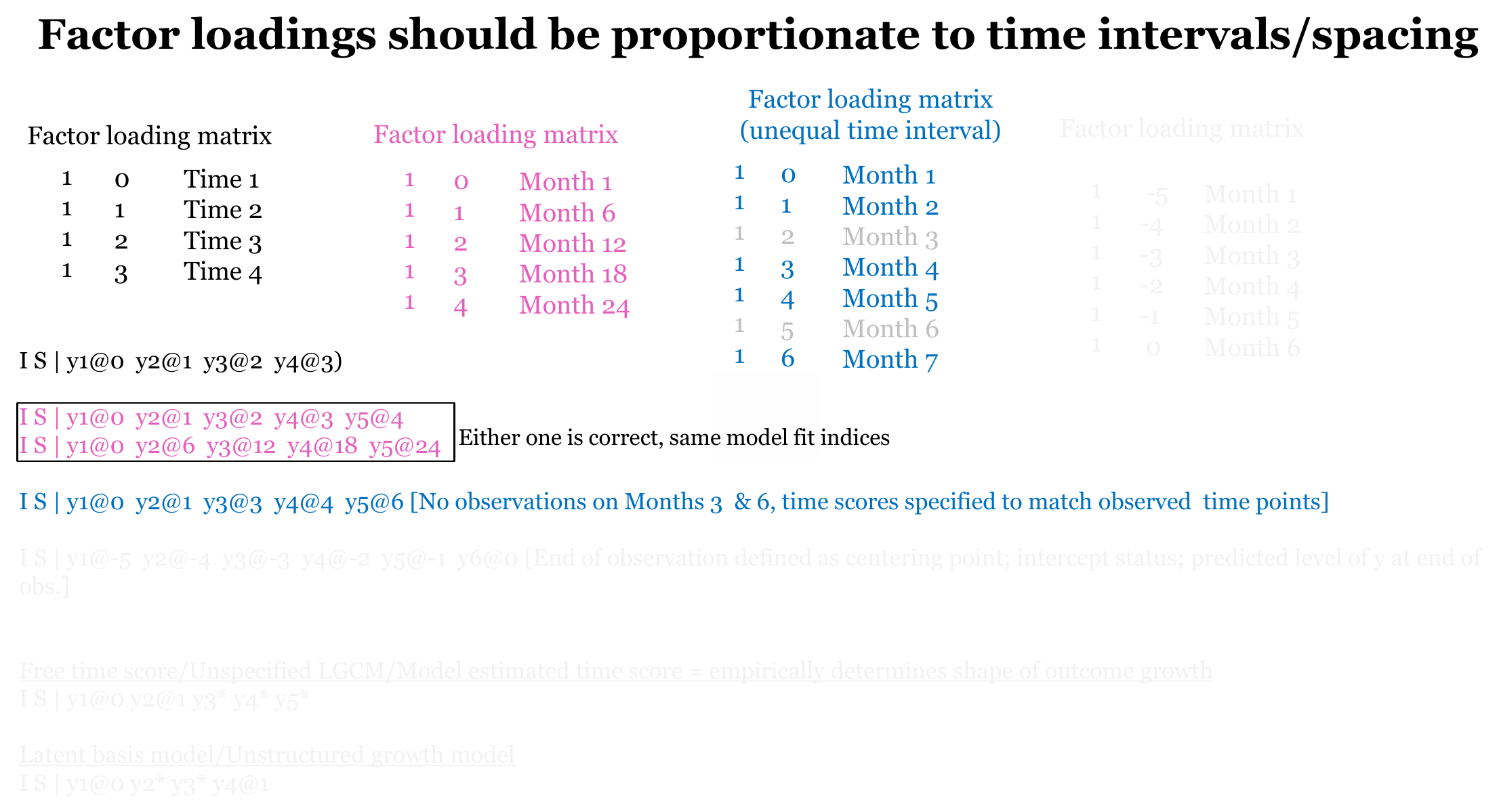
If the waves were equally spaced, the time scores would be 0, 1, 2, 3 and 4. In this dataset the waves are in 2015, 2016, 2018, 2019 and 2021. The gaps are 1, 2, 1 and 2 years. We use 2015 as time 0 and count in years, so the time scores are 0, 1, 3, 4 and 6. Years 2017 and 2020, which correspond to the time scores 2 and 5, were not measured. They do not need a variable in the model, but they take their place on the time axis.
Figure 1.6 makes the same point. The loadings must be proportional to the time intervals. When the waves are equally spaced, any set of equally spaced numbers gives the same fit, for instance 0, 1, 2, 3, 4 or 0, 6, 12, 18, 24 for the same five waves (the slide uses months as its unit). When there are gaps, the time scores are chosen to match the observed time points, as in the blue example on the slide. In this compendium the unit is the year, and not the month. The faded lines on the slide refer to other options, such as centering at the last wave and freely estimated time scores. We touch on centering below, and we do not fit freely estimated time scores in this chapter.
Figure 1.6: Factor loadings proportional to the time intervals. Look at the blue example, where no observations exist at two of the time points and the time scores are specified to match the observed time points. Source: workshop slides (Anyan, 2023).
1.6.3 The formal model
For participant \(i\) at time score \(\lambda_t\), the linear growth model with an intercept factor and a slope factor is
with \((\lambda_1, \dots, \lambda_5) = (0, 1, 3, 4, 6)\). The mean of the repeated measure at time \(t\) is \(\alpha_0 + \lambda_t \alpha_1\). The parameter \(\alpha_0\) is the mean of the intercept factor, \(\alpha_1\) is the mean of the slope factor, and the variances and covariance of \(\zeta_{0i}\) and \(\zeta_{1i}\) describe how participants differ. The time scores are fixed numbers. They enter as the second column of the loading matrix, and the first column is a column of ones. Changing them changes the model-implied means and covariances in a way that depends on the time points and not on the number of the wave.
1.6.4 Checking the effect of the coding
The data do not tell lavaan which time scores are correct. The model runs with any numbers that you give it. To see what the coding changes, we fit the linear model with four sets of time scores. The first is the workshop coding. The second is a coding that treats the waves as equally spaced, which does not match the design. The third centers time at 2021. The fourth keeps the spacing of the workshop but divides the time scores by six, so that one unit is the whole period from 2015 to 2021. The chunk is an addition to the workshop. The function builds the model string from the time scores, and the workshop syntax for the linear model is the first row.
Code
# Addition (not in the workshop): the linear model under different time scoresfit_with_scores <-function(scores) { mod <-paste0("i =~ ", paste0("1*", lone, collapse =" + "), "\n","s =~ ", paste0(scores, "*", lone, collapse =" + "))growth(mod, data = data)}codings <-list("0, 1, 3, 4, 6 (workshop)"=c(0, 1, 3, 4, 6),"0, 1, 2, 3, 4 (equal spacing)"=c(0, 1, 2, 3, 4),"-6, -5, -3, -2, 0 (centered 2021)"=c(-6, -5, -3, -2, 0),"0, 1/6, 3/6, 4/6, 1 (scaled)"=c(0, 1, 3, 4, 6) /6)code_tab <-t(sapply(codings, function(sc) { fit <-fit_with_scores(sc)c(chisq =unname(fitMeasures(fit, "chisq")),cfi =unname(fitMeasures(fit, "cfi")),intercept_mean =get_est(fit, "i", "~1"),slope_mean =get_est(fit, "s", "~1"),intercept_var =get_est(fit, "i", "~~", "i"),slope_var =get_est(fit, "s", "~~", "s"),cov_i_s =get_est(fit, "i", "~~", "s"))}))knitr::kable(code_tab, digits =3)
chisq
cfi
intercept_mean
slope_mean
intercept_var
slope_var
cov_i_s
0, 1, 3, 4, 6 (workshop)
75.244
0.852
1.466
-0.025
0.139
0.003
-0.015
0, 1, 2, 3, 4 (equal spacing)
75.355
0.852
1.467
-0.037
0.144
0.008
-0.024
-6, -5, -3, -2, 0 (centered 2021)
75.244
0.852
1.317
-0.025
0.076
0.003
0.005
0, 1/6, 3/6, 4/6, 1 (scaled)
75.244
0.852
1.466
-0.149
0.139
0.119
-0.091
The workshop coding reproduces the linear model of Chapter 2, with a chi-square of 75.24, an intercept mean of 1.466 and a slope mean of -0.025. The equal spacing coding gives a chi-square of 75.36, which is almost the same. In these data the fit does not reveal that the coding is wrong. The slope mean, however, is -0.037, and it is now a change per wave and not per year. If this value were reported as a change per year, it would be larger than the change per year of the workshop coding by a factor of about 1.48, and the variance of the slope would also be about 2.30 times larger. Centering at 2021 leaves the chi-square and the slope mean unchanged and moves the intercept mean to 1.317, the expected level in 2021. The intercept variance is 0.076 against 0.139 in 2015, and the covariance between the intercept and the slope is 0.005 against -0.015. The sign of that covariance depends on where time is centered. Dividing the time scores by six leaves the fit and the intercept unchanged and multiplies the slope mean by six, so that it becomes the expected change over the whole period, -0.149.
A wrong coding of time still runs
Writing 0*lone1 + 1*lone2 + 2*lone3 + 3*lone4 + 4*lone5 in lavaan gives a model that converges and reports ordinary fit statistics. Nothing in the output says that the loadings do not match the spacing of the waves. The correct time scores come from the study design and the dates of the measurements, and you must check them yourself.
1.7 Measurement before meaning
A growth model for observed scores treats the score at wave 5 as the same measure as the score at wave 1. If the instrument works differently at different waves, a change in the means may reflect a change in measurement as well as a change in the construct. Two properties are relevant, and they are separate. Reliability concerns how much of the variance of a score at one wave is random measurement error. Coefficient alpha is one of the estimates of internal consistency (Cronbach, 1951). It is computed from the items of a scale at a given wave, and it says nothing about stability over time. Measurement invariance over time asks whether the same items relate to the same construct in the same way at each wave. Meredith (1993) described levels of invariance that he called weak, strong and strict. The labels configural, metric and scalar are used in later work, and the usual conventions for testing and reporting them are reviewed by Putnick & Bornstein (2016). With scalar invariance, the difference between the latent means at two waves is usually taken to reflect a difference in the construct. Without it, that interpretation is less secure.
The dataset in this compendium has one observed score per construct and wave. It does not contain the separate items, so neither reliability nor invariance can be computed from it. In the linear model of Chapter 2 the residual variance at each wave combines measurement error with variation that is specific to that wave, and the model cannot separate the two. When you plan your own analysis, collect the information on the items, and compute the reliability at each wave. Test invariance over time on the items before you fit a growth model to scores built from them. In the dataset of this compendium, we treat the scores as comparable across the waves. This is an assumption, and we do not test it.
Report what was checked
State in the text which properties of the measures were examined before the growth model, and which were assumed. A sentence on the reliability at each wave and on the invariance over time is enough in most articles.
1.8 Researcher’s perspective
The checks in this chapter lead to decisions that you should report together with the models.
Report the number of participants in the data and the number that each model used. In this dataset the loneliness models use 321 of 442 participants under the default settings.
State how missing data were handled and why. Give the missing data pattern, state the assumption behind the method, and report a sensitivity analysis when the handling could matter. Here the means of the growth factors changed little between listwise deletion and FIML, while the variances and the fit indices changed more.
Describe the distributions. With skewness as large as in this dataset, the standard errors and the chi-square based fit indices are less certain, and the MLR estimator is an alternative to consider.
Give the time scores, their unit and the point at which time is centered, with the reason for choosing them.
Report which parts of measurement were checked and which were assumed.
From the descriptive work in this chapter we expect an average that is somewhat lower at the end than at the start, relative standing that is moderately stable and fades with distance in time, and visible differences between individual trajectories. These are expectations. Chapter 2 fits the first models and compares which form of change the data support.
Anyan, F. (2023). Longitudinal data analysis using Mplus and R. Workshop slides.
Baltes, P. B., & Nesselroade, J. R. (1979). History and rationale of longitudinal research. In J. R. Nesselroade & P. B. Baltes (Eds.), Longitudinal research in the study of behavior and development (pp. 1–39). Academic Press.
Biesanz, J. C., Deeb-Sossa, N., Papadakis, A. A., Bollen, K. A., & Curran, P. J. (2004). The role of coding time in estimating and interpreting growth curve models. Psychological Methods, 9(1), 30–52. https://doi.org/10.1037/1082-989X.9.1.30
Cronbach, L. J. (1951). Coefficient alpha and the internal structure of tests. Psychometrika, 16(3), 297–334. https://doi.org/10.1007/BF02310555
Curran, P. J., Obeidat, K., & Losardo, D. (2010). Twelve frequently asked questions about growth curve modeling. Journal of Cognition and Development, 11(2), 121–136. https://doi.org/10.1080/15248371003699969
Curran, P. J., West, S. G., & Finch, J. F. (1996). The robustness of test statistics to nonnormality and specification error in confirmatory factor analysis. Psychological Methods, 1(1), 16–29. https://doi.org/10.1037/1082-989X.1.1.16
Enders, C. K. (2010). Applied missing data analysis. Guilford Press.
Enders, C. K., & Bandalos, D. L. (2001). The relative performance of full information maximum likelihood estimation for missing data in structural equation models. Structural Equation Modeling: A Multidisciplinary Journal, 8(3), 430–457. https://doi.org/10.1207/S15328007SEM0803_5
Hu, L., & Bentler, P. M. (1999). Cutoff criteria for fit indexes in covariance structure analysis: Conventional criteria versus new alternatives. Structural Equation Modeling: A Multidisciplinary Journal, 6(1), 1–55. https://doi.org/10.1080/10705519909540118
McArdle, J. J. (2012). Foundational issues in the contemporary modeling of longitudinal trajectories. In B. Laursen, T. D. Little, & N. A. Card (Eds.), Handbook of developmental research methods (pp. 385–410). Guilford Press.
Meredith, W. (1993). Measurement invariance, factor analysis and factorial invariance. Psychometrika, 58(4), 525–543. https://doi.org/10.1007/BF02294825
Putnick, D. L., & Bornstein, M. H. (2016). Measurement invariance conventions and reporting: The state of the art and future directions for psychological research. Developmental Review, 41, 71–90. https://doi.org/10.1016/j.dr.2016.06.004
R Core Team. (2024). R: A language and environment for statistical computing. R Foundation for Statistical Computing. https://www.R-project.org/
Revelle, W. (2024). psych: Procedures for psychological, psychometric, and personality research (Version 2.4.1). Northwestern University. https://CRAN.R-project.org/package=psych
Rosseel, Y. (2012). lavaan: An R package for structural equation modeling. Journal of Statistical Software, 48(2), 1–36. https://doi.org/10.18637/jss.v048.i02
Wickham, H. (2016). ggplot2: Elegant graphics for data analysis. Springer-Verlag New York. https://ggplot2.tidyverse.org
Wickham, H., François, R., Henry, L., Müller, K., & Vaughan, D. (2023). dplyr: A grammar of data manipulation (Version 1.1.4). https://CRAN.R-project.org/package=dplyr
Yuan, K.-H., & Bentler, P. M. (2000). Three likelihood-based methods for mean and covariance structure analysis with nonnormal missing data. Sociological Methodology, 30, 165–200.
Source Code
# Practical preliminaries before fitting growth models {#sec-prelims}```{r}#| label: setup#| include: falselibrary(lavaan)library(dplyr)library(tidyr)library(ggplot2)library(psych)data <-read.csv("data/data.csv", fileEncoding ="UTF-8-BOM")theme_set(theme_minimal(base_size =12) +theme(plot.title =element_text(face ="bold", color ="black"),axis.title =element_text(color ="black"),axis.text =element_text(color ="black"),strip.text =element_text(color ="black"),legend.text =element_text(color ="black")))# small helpers for inline numbersf2 <-function(x) formatC(x, format ="f", digits =2)f1 <-function(x) formatC(x, format ="f", digits =1)f3 <-function(x) formatC(x, format ="f", digits =3)fp <-function(p) sub("^0", "", formatC(p, format ="f", digits =2))fp3 <-function(p) sub("^0", "", formatC(p, format ="f", digits =3))fv <-function(x, d =2) paste(formatC(x, format ="f", digits = d), collapse =", ")lone <-paste0("lone", 1:5)anx <-paste0("anx", 1:5)dep <-paste0("dep", 1:5)host <-paste0("host", 1:5)```The syntax of `growth()` in lavaan is short and the models run in seconds. R returns fit statistics whether or not the time scores or the missing data make sense. Thus, we check these first. This chapter collects the checks that come before the first `=~` line.There is no growth model in this chapter. We use R [@rcoreteam], psych [@revelle2024psych], dplyr [@wickham2023dplyr], tidyr [@wickham2024tidyr] and ggplot2 [@wickham2016ggplot2] to describe the data, and we use lavaan [@rosseel2012lavaan] for one small robustness run on the missing data. The models start in @sec-basic. Throughout the compendium we work with one dataset of `r nrow(data)` rows and `r ncol(data)` columns. Loneliness (`lone1` to `lone5`), anxiety symptoms (`anx1` to `anx5`), depression symptoms (`dep1` to `dep5`) and hostility (`host1` to `host5`) were measured at five waves, in 2015, 2016, 2018, 2019 and 2021. We use loneliness as the running example in this chapter. Every step applies in the same way to the other three variables.## Why look at the data firstThe objectives of longitudinal research include describing change within persons and describing differences between persons in that change [@baltes1979history]. A growth model addresses both objectives. The trajectory that it describes depends on the form and the time scores that you give it, and the foundational issues in modeling trajectories are discussed by @mcardle2012latent. If the form or the time scores are wrong, the model still returns numbers. For this reason, we look at the data before we model them.The preliminary work answers four questions.i. What does the average trajectory look like?ii. How stable is the relative standing of participants from one wave to the next?iii. How much information is missing, and where?iv. How are the waves spaced in time?These questions can be answered with descriptive statistics, correlations, a missing data table and plots, and no latent variable is needed.## Descriptive statistics for each wave### The idea in plain languageBefore we ask whether individuals change, we ask what the sample looks like at each wave. Flat sample means speak against a strong linear trend. Means that rise or fall steadily suggest that a straight line is a reasonable starting point. Means that rise and then fall suggest that one constant rate of change may not be enough. We also look at the shape of the distributions, because the estimation method in the workshop assumes multivariate normality.### R implementationThe function `describe()` from psych returns the number of observed values, the mean, the standard deviation and the shape of the distribution for each wave in one call.```{r}#| label: prelims-descriptives-lone# Number of observed values, mean, standard deviation and shape of the distribution for each wavedesc_lone <-describe(data[, lone])desc_lonedesc_all <-describe(data[, c(lone, anx, dep)])``````{r}#| label: prelims-descriptives-complete-cases# Wave means for the participants who are complete on all five wavescc_lone <-complete.cases(data[, lone])round(colMeans(data[cc_lone, lone]), 2)# Addition: paired test of the change from the first to the third wave, complete casestt13 <-t.test(data$lone3[cc_lone], data$lone1[cc_lone], paired =TRUE)c(mean_diff =unname(tt13$estimate), t =unname(tt13$statistic), p = tt13$p.value)```### Understanding the outputThe number of observed values differs between the waves. The scores are observed for `r paste(desc_lone$n, collapse = ", ")` of the `r nrow(data)` participants at the five waves. This is the first sign of missing data, which the next section examines.The means are `r fv(desc_lone$mean)` for 2015, 2016, 2018, 2019 and 2021. The mean is `r f2(desc_lone$mean[3] - desc_lone$mean[1])` higher in 2018 than in 2015, and it is lower in the last two waves. The mean in 2021 is `r f2(desc_lone$mean[1] - desc_lone$mean[5])` lower than the mean in 2015. The standard errors of the wave means are `r fv(desc_lone$se, 3)`. The means for the `r sum(cc_lone)` participants with complete data are given by the second chunk, and they show the same pattern. Among these participants the rise from 2015 to 2018 is `r f2(tt13$estimate)` (paired *t* = `r f2(tt13$statistic)`, *p* = `r fp3(tt13$p.value)`). It is small in size but distinguishable from zero, at about `r f1(tt13$statistic)` standard errors. Thus, the average level is lower in 2021 than in 2015. The shape of the path is examined with the models.The standard deviations are `r fv(desc_lone$sd)`. The spread is smaller at the last wave. In a score with most values near the lowest observed value, a smaller spread can reflect a floor effect as much as a change in how much participants differ. For that reason we do not read the standard deviations as evidence about individual differences in change. The variances of the growth factors address this more directly.The shape of the distributions matters as well. The lowest observed value is `r fv(unique(desc_lone$min), 0)` at every wave and the medians are between `r f2(min(desc_lone$median))` and `r f2(max(desc_lone$median))`. Thus, most participants score close to the bottom of the range and a few score much higher. The skewness is between `r f2(min(desc_lone$skew))` and `r f2(max(desc_lone$skew))` and the kurtosis is between `r f2(min(desc_lone$kurtosis))` and `r f2(max(desc_lone$kurtosis))`. Across the `r length(c(lone, anx, dep))` loneliness, anxiety and depression scores, the skewness ranges from `r f2(min(desc_all$skew))` to `r f2(max(desc_all$skew))`.Maximum likelihood, the default estimator in `growth()`, assumes that the observed variables are multivariate normal. With distributions as skewed as these, this assumption is doubtful. In a simulation study of confirmatory factor analysis, the maximum likelihood chi-square was inflated when the data were non-normal [@curran1996robustness]. That study does not cover growth models, so we take it as a reason for caution and not as a measure of the bias here. Standard errors can be affected as well. The robust version of maximum likelihood, called MLR in lavaan, gives standard errors and a scaled chi-square statistic that account for non-normality [@yuan2000three]. We use it for one check in the section on missing data. The fit indices in the later chapters should be read with this caution in mind.## Correlations across waves### The idea in plain languageThe wave means describe the sample as a whole. The correlations between waves describe the relative standing of participants. A participant who is comparatively high at one wave can stay comparatively high at later waves, or the ordering of participants can change. The means and the ordering of participants can change independently. A growth model represents both aspects. The means of the growth factors describe the average trajectory, and the variances of the growth factors describe how much participants differ in their starting point and their rate of change.If a score were a stable characteristic with a little random noise, all pairs of waves would correlate about equally, whatever the distance between them. If the correlations become smaller as the time between the waves increases, relative standing may be changing gradually, and that would leave room for individual differences in change. The variance of a slope factor captures such differences. An autoregressive process or wave-specific variance can produce the same pattern, so the correlations alone do not settle the matter.### R implementation```{r}#| label: prelims-correlations-loneround(cor(data[, lone], use ="pairwise.complete.obs"), 2)```The following chunk is an addition to the workshop. It lists the same correlations next to the number of years between the two waves, because the waves are not equally spaced.```{r}#| label: prelims-correlations-by-gap# Addition: correlations ordered by the distance in years between the two wavesr_lone <-cor(data[, lone], use ="pairwise.complete.obs")years <-c(0, 1, 3, 4, 6)idx <-which(upper.tri(r_lone), arr.ind =TRUE)gap_tab <-data.frame(pair =paste(lone[idx[, 1]], lone[idx[, 2]], sep =" - "),years_apart =abs(years[idx[, 1]] - years[idx[, 2]]),r =round(r_lone[idx], 2))gap_tab[order(gap_tab$years_apart, -gap_tab$r), ]```### Understanding the outputThe correlations are positive in every pair and they lie between `r f2(min(r_lone[upper.tri(r_lone)]))` and `r f2(max(r_lone[upper.tri(r_lone)]))`. The pairs that are one year apart (`lone1` and `lone2`, `lone3` and `lone4`) correlate at `r f2(r_lone[1, 2])` and `r f2(r_lone[3, 4])`. The two pairs that are two years apart correlate at `r f2(r_lone[2, 3])` and `r f2(r_lone[4, 5])`, and the pair that is six years apart (`lone1` and `lone5`) correlates at `r f2(r_lone[1, 5])`, which is the lowest value in the matrix. Notice that adjacent waves are not equally far apart. The correlations decrease with the years between the waves, although not perfectly. The pair `lone3` and `lone4` is one year apart and correlates at `r f2(r_lone[3, 4])`, which is lower than the pair `lone2` and `lone3` at two years apart (`r f2(r_lone[2, 3])`).The correlations are computed on all pairs of available values, so they rest on different numbers of participants. They are not the same as the correlations among the `r sum(cc_lone)` complete cases that the models use.### InterpretationThe pattern is consistent with moderate stability of relative standing that fades slowly with time. No correlation is near zero, so participants who are comparatively high at the start tend to remain comparatively high. No correlation is near one. This is compatible with participants changing at different rates, but correlations that decrease with distance also arise from wave-specific variation or an autoregressive process, and a correlation matrix does not separate these from systematic change. A slope factor with some variance is therefore something to look for in @sec-basic, and the correlations do not establish it.## Missing data### How much is missing, and whereEvery number above rests on whichever participants have data at that wave. Before we trust a model we need to know how much data is missing and in what pattern. This section is the one place in the compendium where listwise deletion, full information maximum likelihood (FIML) and the missing at random assumption are explained in full. The later chapters report the number of participants that each model used, give a short sensitivity result and refer to this section.```{r}#| label: prelims-missingnesscolSums(is.na(data))``````{r}#| label: prelims-missing-patternsn_complete_lone <-sum(complete.cases(data[, lone]))n_complete_cov <-sum(complete.cases(data[, c("female", host)]))cat("Complete on all five loneliness waves:", n_complete_lone, "of", nrow(data), "\n")cat("Complete on female and all five hostility waves:", n_complete_cov, "of", nrow(data), "\n")# Number of waves with an observed loneliness score, per participantn_waves <-rowSums(!is.na(data[, lone]))table(n_waves)# Is a participant missing the same waves on all four measures?same_rows <-all(sapply(1:5, function(w) { m <-is.na(data[[paste0("lone", w)]])all(m ==is.na(data[[paste0("anx", w)]]) & m ==is.na(data[[paste0("dep", w)]]) & m ==is.na(data[[paste0("host", w)]]))}))same_rows# Participants with a missing wave that is followed by an observed waven_gap <-sum(apply(!is.na(data[, lone]), 1, function(o) any(!o[-5] &sapply(1:4, function(k) any(o[(k +1):5])))))n_gap```The number of missing values on the loneliness scores is `r paste(colSums(is.na(data[, lone])), collapse = ", ")` at the five waves. `r ifelse(same_rows, "At every wave, the same participants are missing on all four repeated measures, which is why the counts for anx, dep and host repeat those of lone.", "The participants who are missing differ between the four repeated measures.")` Of the `r nrow(data)` rows, `r n_complete_lone` have data at all five waves on loneliness (`r f1(100 * n_complete_lone / nrow(data))` percent), and `r n_complete_cov` have complete data on `female` and the five hostility scores. Further, `r sum(n_waves == 0)` participants have no loneliness data at any wave. The variable `female` is missing for `r sum(is.na(data$female))` participants, and the substance use score `subs5`, measured only at the last wave, is missing for `r sum(is.na(data$subs5))` participants (`r f1(100 * sum(is.na(data$subs5)) / nrow(data))` percent), which is the largest count of any variable. The variables `pdu1` and `ace1` are missing for `r sum(is.na(data$pdu1))` participants each. They are not used in the models of this compendium.The table of the number of observed waves shows that most participants with missing values still have data at several waves. The missing values are also not only the result of participants leaving the study. For `r n_gap` participants a missing wave is followed by a later wave with data. Several mechanisms can produce such patterns, and the dataset does not tell us which one operated.### What the workshop script doesThe workshop script calls `growth()` with its default settings. The default for missing data in lavaan is listwise deletion, so a participant who is missing on any of the variables in the model is removed before estimation. For the loneliness models this leaves `r n_complete_lone` of `r nrow(data)` participants, and lavaan reports it in the line "Used" and "Total" in the summary. The models that include covariates or an outcome measured once use fewer participants, and the multigroup models also drop the participants with missing `female`. In that case lavaan prints the message that the group variable contains missing values. Take the number of participants that a model used from the lavaan output and not from the number of rows in the dataset.Listwise deletion is simple to apply and to report. It costs power, because `r nrow(data) - n_complete_lone` participants (`r f1(100 * (nrow(data) - n_complete_lone) / nrow(data))` percent of the rows) contribute nothing, even though most of them have data at some waves. It can also bias the estimates, if the participants who are dropped differ from those who are kept in ways that are related to the scores [@enders2010applied].### Listwise deletion and full information maximum likelihoodFull information maximum likelihood (FIML) uses every available value. A participant with three observed waves contributes the information of those three waves to the likelihood. In lavaan, FIML is requested with `missing = "fiml"`. Data are missing completely at random when the probability of a missing value is unrelated to any score, observed or not. They are missing at random (MAR) when this probability depends on observed values only, and missing not at random when it depends on the missing value itself, given the observed ones [@rubin1976inference]. FIML gives valid estimates under MAR and under missing completely at random. Listwise deletion is valid only under the latter. In the simulation conditions that @enders2001relative examined, FIML was found to perform better than listwise deletion in structural equation models. @enders2010applied gives a full treatment. FIML as implemented in lavaan also assumes multivariate normality, so the caution about non-normality above applies to it as well.Missing at random cannot be verified from the data, because the assumption concerns the values that we did not observe. We can only look for signs that the participants who are missing differ on what we do observe. The following chunk is an addition to the workshop. It compares the first loneliness score of the participants who have data at all five waves with that of the participants who have the first score but are missing at a later wave.```{r}#| label: prelims-attrition-check# Addition: initial loneliness for complete versus incomplete participantsinc <-!cc_lone &!is.na(data$lone1)tt <-t.test(data$lone1[inc], data$lone1[cc_lone])c(n_incomplete =sum(inc), mean_incomplete =mean(data$lone1[inc]),n_complete =sum(cc_lone), mean_complete =mean(data$lone1[cc_lone]),p = tt$p.value)```The `r sum(inc)` participants who have a first score but are missing later have a mean of `r f2(mean(data$lone1[inc]))` at the first wave, against `r f2(mean(data$lone1[cc_lone]))` for the `r sum(cc_lone)` complete participants. The difference is small relative to its uncertainty (*p* = `r fp(tt$p.value)`). This suggests that there is no large difference in initial level between the two groups. It does not show that the data are missing at random, since the later values of those who left are not observed, and a test with `r sum(inc)` participants has limited power.::: {.callout-note title="Missing at random is an assumption"}A table of missing values and a comparison of observed scores cannot prove that the missing values are missing at random. They can only show that nothing in the observed data contradicts it. Whether a method is justified depends on reasons for missingness that lie outside the data, so state the assumption when you report the method.:::### Sensitivity to the missing data handlingThe workshop models are fitted with listwise deletion, and those are the numbers reported in the chapters. To see how much the handling of missing data matters, we fit the linear model of @sec-basic twice, once with the default and once with FIML. The model syntax in the chunk below is the workshop syntax and has not been changed. The lines that request FIML, and everything that follows in this subsection, are an addition that was not part of the workshop.```{r}#| label: prelims-fiml-sensitivitylinear <-' i =~ 1*lone1 + 1*lone2 + 1*lone3 + 1*lone4 + 1*lone5 s =~ 0*lone1 + 1*lone2 + 3*lone3 + 4*lone4 + 6*lone5'fit_linear_lw <-growth(linear, data = data)# Addition (not in the workshop): the same model with FIMLfit_linear_fiml <-growth(linear, data = data, missing ="fiml")```The warning that lavaan prints for the FIML model says that some cases are empty and will be ignored. These are the participants without a single loneliness score. They cannot contribute to the likelihood of a model for these five variables, and there are `r sum(n_waves == 0)` of them. With FIML the model uses `r lavInspect(fit_linear_fiml, "nobs")` participants. With listwise deletion it uses `r lavInspect(fit_linear_lw, "nobs")`.```{r}#| label: prelims-fiml-tableget_est <-function(fit, lhs, op, rhs ="") { pe <-parameterEstimates(fit) pe$est[pe$lhs == lhs & pe$op == op & pe$rhs == rhs]}tab_one <-function(fit) {c(n_used =lavInspect(fit, "nobs"),intercept_mean =get_est(fit, "i", "~1"),slope_mean =get_est(fit, "s", "~1"),intercept_var =get_est(fit, "i", "~~", "i"),slope_var =get_est(fit, "s", "~~", "s"),covariance_i_s =get_est(fit, "i", "~~", "s"),chisq =unname(fitMeasures(fit, "chisq")),cfi =unname(fitMeasures(fit, "cfi")),rmsea =unname(fitMeasures(fit, "rmsea")),srmr =unname(fitMeasures(fit, "srmr")))}sens <-data.frame(listwise =tab_one(fit_linear_lw), fiml =tab_one(fit_linear_fiml))knitr::kable(sens, digits =3)``````{r}#| label: prelims-mlr-check# Addition: FIML with robust (MLR) standard errors and scaled test statisticfit_linear_mlr <-growth(linear, data = data, missing ="fiml", estimator ="MLR")round(fitMeasures(fit_linear_mlr, c("chisq.scaled", "df.scaled", "cfi.robust", "rmsea.robust")), 3)```The mean of the intercept factor is `r f3(sens["intercept_mean", "listwise"])` with listwise deletion and `r f3(sens["intercept_mean", "fiml"])` with FIML. The mean of the slope factor is `r f3(sens["slope_mean", "listwise"])` and `r f3(sens["slope_mean", "fiml"])`. Hence, the estimated average starting level and the estimated average yearly change move little. The variances are somewhat larger with FIML. The intercept variance is `r f3(sens["intercept_var", "listwise"])` against `r f3(sens["intercept_var", "fiml"])`, and the slope variance is `r f3(sens["slope_var", "listwise"])` against `r f3(sens["slope_var", "fiml"])`. In both runs the covariance between the intercept and slope factors is negative, and the slope variance is small but above zero.The fit looks better with FIML (CFI `r f3(sens["cfi", "fiml"])` against `r f3(sens["cfi", "listwise"])`, RMSEA `r f3(sens["rmsea", "fiml"])` against `r f3(sens["rmsea", "listwise"])`). The two fit statistics are not strictly comparable, because they come from different numbers of participants. Neither set reaches the combination rules that are commonly used for these indices [@hu1999cutoff]. The robust run gives a scaled chi-square of `r f2(fitMeasures(fit_linear_mlr, "chisq.scaled"))` on `r fitMeasures(fit_linear_mlr, "df.scaled")` degrees of freedom, against `r f2(sens["chisq", "fiml"])` for the standard FIML statistic, with CFI `r f3(fitMeasures(fit_linear_mlr, "cfi.robust"))` and RMSEA `r f3(fitMeasures(fit_linear_mlr, "rmsea.robust"))`. A smaller scaled statistic is in line with an inflated standard chi-square under non-normality, but the fit remains short of the usual benchmarks.In short, the substantive reading of the linear model does not depend much on how the missing data are handled, but the variances and the fit statistics change more. The FIML result does not remove the uncertainty about the missing data mechanism. It rests on the same missing at random assumption that we cannot test.## Trajectory plots### The idea in plain languageTables of means and correlations average over participants, and two quite different patterns of change can give the same means. Everyone can change in about the same way, or participants can differ a lot and cancel out on average. A plot with all participants shows the overall form and whether there are obvious clusters. A small set of individual panels shows what single trajectories look like.### R implementationThe scores are first rearranged from wide to long format, with one row per participant and wave.```{r}#| label: fig-prelims-sample#| fig-cap: "Individual loneliness trajectories (thin blue lines) with the sample mean trend overlaid (thick red line)."#| fig-alt: "Thin blue lines for each participant across five waves, with a thick red line for the mean at each wave."#| warning: falselong_lone <- data %>%select(personid, lone1, lone2, lone3, lone4, lone5) %>%pivot_longer(cols =starts_with("lone"), names_to ="wave", values_to ="loneliness") %>%mutate(wave_num =as.numeric(gsub("lone", "", wave)),loneliness =suppressWarnings(as.numeric(loneliness)))ggplot(long_lone, aes(x = wave_num, y = loneliness, group = personid)) +geom_line(alpha =0.15, color ="#1f4e79") +stat_summary(aes(group =1), fun = mean, geom ="line", linewidth =1.4, color ="#c0392b") +stat_summary(aes(group =1), fun = mean, geom ="point", size =2.2, color ="#c0392b") +scale_x_continuous(breaks =1:5, labels =c("2015", "2016", "2018", "2019", "2021")) +labs(title ="Individual and mean loneliness trajectories",x ="Wave (year)", y ="Loneliness")``````{r}#| label: fig-prelims-individual#| fig-cap: "Individual trajectories for 12 randomly sampled participants."#| fig-alt: "Twelve small panels, each with the five loneliness scores of one participant joined by a line."#| fig-width: 8#| fig-height: 5.5#| warning: falseset.seed(42)sample_ids <-sample(unique(long_lone$personid), 12)long_lone %>%filter(personid %in% sample_ids) %>%ggplot(aes(x = wave_num, y = loneliness)) +geom_line(color ="#1f4e79") +geom_point(color ="#1f4e79") +facet_wrap(~personid, ncol =4) +scale_x_continuous(breaks =1:5, labels =c("15", "16", "18", "19", "21")) +labs(title ="Individual trajectories: 12 randomly sampled participants",x ="Wave (year)", y ="Loneliness")```Both plots place the five waves at equal distances on the horizontal axis, and the labels give the year. This is convenient for a first look, but it hides the unequal spacing of the waves. The next chunk is an addition to the workshop. It plots the wave means at their real position on the time axis. The vertical axis starts at 1, the lowest observed value, so that the differences between the means are not exaggerated.```{r}#| label: fig-prelims-means-years#| fig-cap: "Mean loneliness at each wave, placed at the year of measurement."#| fig-alt: "Five points for the wave means placed at 2015, 2016, 2018, 2019 and 2021 and joined by line segments, on a vertical axis from 1 to 2."#| fig-width: 6#| fig-height: 3.5#| warning: false# Addition: wave means at the real calendar positionmean_tab <-data.frame(year =c(2015, 2016, 2018, 2019, 2021),mean_lone =colMeans(data[, lone], na.rm =TRUE))ggplot(mean_tab, aes(x = year, y = mean_lone)) +geom_line(color ="#c0392b") +geom_point(color ="#c0392b", size =2.2) +scale_x_continuous(breaks =2015:2021) +scale_y_continuous(limits =c(1, 2)) +labs(title ="Wave means at the year of measurement", x ="Year", y ="Mean loneliness")```### Understanding the output@fig-prelims-sample shows a dense cloud of lines, and a mean line that follows the numbers in the descriptive table. A participant with a missing wave shows a gap in the line. The mean is computed from the observed values at each wave. The cloud does not separate into two obvious bundles, so there is no sign in this plot that the participants form clearly distinct groups. The lines are bunched near the bottom of the score range and a minority of participants reach much higher values, which agrees with the skewness reported earlier.@fig-prelims-individual shows `r length(sample_ids)` participants, drawn at random with `set.seed(42)`, each in a small panel. The panels differ from each other in level and in shape, and several contain gaps because of missing waves. Some participants stay close to the lowest values throughout, one participant peaks at the second wave and then falls, and one falls across the waves. Participants differ in where they start, and they also seem to differ in how their scores move over time. The statement that average loneliness is lower at the end does not describe any of these panels well. Twelve participants are a small sample, so these panels illustrate the variation and do not measure it. The growth models quantify it through the variances of the growth factors.@fig-prelims-means-years places the means on the calendar. The gaps between the waves alternate between one and two years. The distances on this axis are the ones that the time scores must represent.## Time scores### The idea in plain languageA growth model describes how the repeated measures change with time. The model needs to know when each measure was taken, and it receives this information through the loadings of the repeated measures on the slope factor. These loadings are the time scores. @fig-prelims-basic-slide shows the basic model with an intercept factor *I* and a slope factor *S* and four repeated measures. The loadings of the measures on *I* are all 1, and the loadings on *S* are the time scores 0, 1, 2 and 3. The slide comes from the workshop, in which the models were estimated with Mplus and with R. It shows the structure of the model and no estimates. All numbers in this chapter come from the R output.```{r}#| label: fig-prelims-basic-slide#| echo: false#| fig-cap: "The basic growth model with an intercept factor (I) and a slope factor (S). The loadings on I are fixed to 1 and the loadings on S are the time scores. Look at the arrows from S to the measures, which carry the time scores. Source: workshop slides [@anyan2023workshop]."#| fig-alt: "Path diagram with an intercept factor I and a slope factor S, a curved arrow between them, and four observed measures with loadings 1.0 from I and 0.0, 1.0, 2.0 and 3.0 from S"#| out-width: "75%"knitr::include_graphics("images/slides/slide_06.png")```The time scores set the form of the growth process, the centering point and the scaling of the growth factors, as @fig-prelims-roles-slide lists. The right-hand side of the slide shows the same four waves coded in two ways. With the time scores 0, 1, 2 and 3 the intercept factor is the level at the first wave. With the time scores -3, -2, -1 and 0 the intercept factor is the level at the last wave. The slope has the same meaning in both, a change per unit of time, but the intercept and its variance describe a different moment.```{r}#| label: fig-prelims-roles-slide#| echo: false#| fig-cap: "The role of the time scores. Look at the two factor loading matrices on the right. They contain the same model with the intercept placed at the first wave (left matrix) and at the last wave (right matrix). Source: workshop slides [@anyan2023workshop]."#| fig-alt: "Slide listing three roles of time scores (form, centering point, scaling of growth factors) with two factor loading matrices that code four waves as 0 to 3 and as -3 to 0"#| out-width: "90%"knitr::include_graphics("images/slides/slide_09.png")```The pattern of the time scores sets the shape of the trajectory that the factors can represent. Time scores that increase in a straight line give a linear form. The quadratic model in @sec-basic uses a third factor whose loadings are the squares of the time scores. The models in @sec-piecewise use different time scores for different periods.The time score of 0 marks the point where the intercept factor is defined. The mean of the intercept factor is the expected score at that point, and its variance is the variance of the levels at that point. The covariance between the intercept and slope factors also depends on this choice.The unit of the time scores sets the unit of the slope. If the time scores count years, the slope is a change per year. If they count the waves, it is a change per wave. The coding of time changes what the intercept and related parameters mean, and the time scores should follow the actual time metric [@biesanz2004coding]. Practical questions about the metric of time are discussed by @curran2010twelve.### Unequal spacing between the wavesIf the waves were equally spaced, the time scores would be 0, 1, 2, 3 and 4. In this dataset the waves are in 2015, 2016, 2018, 2019 and 2021. The gaps are 1, 2, 1 and 2 years. We use 2015 as time 0 and count in years, so the time scores are 0, 1, 3, 4 and 6. Years 2017 and 2020, which correspond to the time scores 2 and 5, were not measured. They do not need a variable in the model, but they take their place on the time axis.@fig-prelims-spacing-slide makes the same point. The loadings must be proportional to the time intervals. When the waves are equally spaced, any set of equally spaced numbers gives the same fit, for instance 0, 1, 2, 3, 4 or 0, 6, 12, 18, 24 for the same five waves (the slide uses months as its unit). When there are gaps, the time scores are chosen to match the observed time points, as in the blue example on the slide. In this compendium the unit is the year, and not the month. The faded lines on the slide refer to other options, such as centering at the last wave and freely estimated time scores. We touch on centering below, and we do not fit freely estimated time scores in this chapter.```{r}#| label: fig-prelims-spacing-slide#| echo: false#| fig-cap: "Factor loadings proportional to the time intervals. Look at the blue example, where no observations exist at two of the time points and the time scores are specified to match the observed time points. Source: workshop slides [@anyan2023workshop]."#| fig-alt: "Slide showing loading matrices for equally spaced waves, for waves coded in months, and for unequally spaced waves where time scores 0, 1, 3, 4 and 6 are matched to observed time points"#| out-width: "90%"knitr::include_graphics("images/slides/slide_12.png")```### The formal modelFor participant $i$ at time score $\lambda_t$, the linear growth model with an intercept factor and a slope factor is$$y_{ti} = \eta_{0i} + \lambda_t \, \eta_{1i} + \varepsilon_{ti}, \qquad\eta_{0i} = \alpha_0 + \zeta_{0i}, \qquad\eta_{1i} = \alpha_1 + \zeta_{1i},$$with $(\lambda_1, \dots, \lambda_5) = (0, 1, 3, 4, 6)$. The mean of the repeated measure at time $t$ is $\alpha_0 + \lambda_t \alpha_1$. The parameter $\alpha_0$ is the mean of the intercept factor, $\alpha_1$ is the mean of the slope factor, and the variances and covariance of $\zeta_{0i}$ and $\zeta_{1i}$ describe how participants differ. The time scores are fixed numbers. They enter as the second column of the loading matrix, and the first column is a column of ones. Changing them changes the model-implied means and covariances in a way that depends on the time points and not on the number of the wave.### Checking the effect of the codingThe data do not tell lavaan which time scores are correct. The model runs with any numbers that you give it. To see what the coding changes, we fit the linear model with four sets of time scores. The first is the workshop coding. The second is a coding that treats the waves as equally spaced, which does not match the design. The third centers time at 2021. The fourth keeps the spacing of the workshop but divides the time scores by six, so that one unit is the whole period from 2015 to 2021. The chunk is an addition to the workshop. The function builds the model string from the time scores, and the workshop syntax for the linear model is the first row.```{r}#| label: prelims-time-score-codings# Addition (not in the workshop): the linear model under different time scoresfit_with_scores <-function(scores) { mod <-paste0("i =~ ", paste0("1*", lone, collapse =" + "), "\n","s =~ ", paste0(scores, "*", lone, collapse =" + "))growth(mod, data = data)}codings <-list("0, 1, 3, 4, 6 (workshop)"=c(0, 1, 3, 4, 6),"0, 1, 2, 3, 4 (equal spacing)"=c(0, 1, 2, 3, 4),"-6, -5, -3, -2, 0 (centered 2021)"=c(-6, -5, -3, -2, 0),"0, 1/6, 3/6, 4/6, 1 (scaled)"=c(0, 1, 3, 4, 6) /6)code_tab <-t(sapply(codings, function(sc) { fit <-fit_with_scores(sc)c(chisq =unname(fitMeasures(fit, "chisq")),cfi =unname(fitMeasures(fit, "cfi")),intercept_mean =get_est(fit, "i", "~1"),slope_mean =get_est(fit, "s", "~1"),intercept_var =get_est(fit, "i", "~~", "i"),slope_var =get_est(fit, "s", "~~", "s"),cov_i_s =get_est(fit, "i", "~~", "s"))}))knitr::kable(code_tab, digits =3)```The workshop coding reproduces the linear model of @sec-basic, with a chi-square of `r f2(code_tab[1, "chisq"])`, an intercept mean of `r f3(code_tab[1, "intercept_mean"])` and a slope mean of `r f3(code_tab[1, "slope_mean"])`. The equal spacing coding gives a chi-square of `r f2(code_tab[2, "chisq"])`, which is almost the same. In these data the fit does not reveal that the coding is wrong. The slope mean, however, is `r f3(code_tab[2, "slope_mean"])`, and it is now a change per wave and not per year. If this value were reported as a change per year, it would be larger than the change per year of the workshop coding by a factor of about `r f2(code_tab[2, "slope_mean"] / code_tab[1, "slope_mean"])`, and the variance of the slope would also be about `r f2(code_tab[2, "slope_var"] / code_tab[1, "slope_var"])` times larger. Centering at 2021 leaves the chi-square and the slope mean unchanged and moves the intercept mean to `r f3(code_tab[3, "intercept_mean"])`, the expected level in 2021. The intercept variance is `r f3(code_tab[3, "intercept_var"])` against `r f3(code_tab[1, "intercept_var"])` in 2015, and the covariance between the intercept and the slope is `r f3(code_tab[3, "cov_i_s"])` against `r f3(code_tab[1, "cov_i_s"])`. The sign of that covariance depends on where time is centered. Dividing the time scores by six leaves the fit and the intercept unchanged and multiplies the slope mean by six, so that it becomes the expected change over the whole period, `r f3(code_tab[4, "slope_mean"])`.::: {.callout-warning title="A wrong coding of time still runs"}Writing `0*lone1 + 1*lone2 + 2*lone3 + 3*lone4 + 4*lone5` in lavaan gives a model that converges and reports ordinary fit statistics. Nothing in the output says that the loadings do not match the spacing of the waves. The correct time scores come from the study design and the dates of the measurements, and you must check them yourself.:::## Measurement before meaningA growth model for observed scores treats the score at wave 5 as the same measure as the score at wave 1. If the instrument works differently at different waves, a change in the means may reflect a change in measurement as well as a change in the construct. Two properties are relevant, and they are separate. Reliability concerns how much of the variance of a score at one wave is random measurement error. Coefficient alpha is one of the estimates of internal consistency [@cronbach1951coefficient]. It is computed from the items of a scale at a given wave, and it says nothing about stability over time. Measurement invariance over time asks whether the same items relate to the same construct in the same way at each wave. @meredith1993measurement described levels of invariance that he called weak, strong and strict. The labels configural, metric and scalar are used in later work, and the usual conventions for testing and reporting them are reviewed by @putnick2016measurement. With scalar invariance, the difference between the latent means at two waves is usually taken to reflect a difference in the construct. Without it, that interpretation is less secure.The dataset in this compendium has one observed score per construct and wave. It does not contain the separate items, so neither reliability nor invariance can be computed from it. In the linear model of @sec-basic the residual variance at each wave combines measurement error with variation that is specific to that wave, and the model cannot separate the two. When you plan your own analysis, collect the information on the items, and compute the reliability at each wave. Test invariance over time on the items before you fit a growth model to scores built from them. In the dataset of this compendium, we treat the scores as comparable across the waves. This is an assumption, and we do not test it.::: {.callout-tip title="Report what was checked"}State in the text which properties of the measures were examined before the growth model, and which were assumed. A sentence on the reliability at each wave and on the invariance over time is enough in most articles.:::## Researcher's perspectiveThe checks in this chapter lead to decisions that you should report together with the models.- Report the number of participants in the data and the number that each model used. In this dataset the loneliness models use `r n_complete_lone` of `r nrow(data)` participants under the default settings.- State how missing data were handled and why. Give the missing data pattern, state the assumption behind the method, and report a sensitivity analysis when the handling could matter. Here the means of the growth factors changed little between listwise deletion and FIML, while the variances and the fit indices changed more.- Describe the distributions. With skewness as large as in this dataset, the standard errors and the chi-square based fit indices are less certain, and the MLR estimator is an alternative to consider.- Give the time scores, their unit and the point at which time is centered, with the reason for choosing them.- Report which parts of measurement were checked and which were assumed.From the descriptive work in this chapter we expect an average that is somewhat lower at the end than at the start, relative standing that is moderately stable and fades with distance in time, and visible differences between individual trajectories. These are expectations. @sec-basic fits the first models and compares which form of change the data support.