In Chapter 1 we looked at the data before fitting anything: the means and spread of the loneliness scores at each wave, the correlations across waves, the missing data, and the choice of time scores. In this chapter we fit the first three growth models to those five waves. We start with the simplest model, in which nothing changes over time, and then add a linear growth model and a quadratic growth model. Each model contains the one before it as a special case, which allows us to ask at every step whether the added part is needed.
2.1 Why start with simple models
A growth model is a statement about how the average level of the outcome moves over time and about how much people differ around that average. We start with the simplest model and add one feature at a time, so each addition answers one question.
The three models in this chapter answer three questions.
Is there a stable level of loneliness and do participants differ in that level, with no systematic change over time? (no growth model)
Does the average level change at a constant rate and do participants differ in their rate of change? (linear growth model)
Does the rate of change itself change over the waves? (quadratic growth model)
The ideas behind these models come from the latent curve framework, in which a growth model is a confirmatory factor model with the loadings tied to time (Meredith & Tisak, 1990). The structural equation perspective is treated in full by Bollen & Curran (2006). Introductions with applied examples are given by Duncan & Duncan (2004) and Preacher et al. (2008). We use the same dataset and the same five waves for all three models, so any difference between them is a difference in the model and not in the data.
2.2 The data and the time scores
The dataset has 442 rows. The loneliness scores lone1 to lone5 were measured at five waves in 2015, 2016, 2018, 2019 and 2021. The gaps between waves are 1, 2, 1 and 2 years, and we therefore use the time scores 0, 1, 3, 4 and 6, with 2015 as time 0 and one unit equal to one year. The reasons were given in Chapter 1. In all three models below, the time scores enter the model as fixed factor loadings.
In the workshop script growth() is called with its default settings, which means listwise deletion. Of the 442 rows, 321 have scores on all five waves, and all three models are estimated on these 321 participants. The output reports this as “Used 321, Total 442”. Listwise deletion, full information maximum likelihood and the missing data assumptions are explained in Chapter 1. The loneliness scores are also skewed (Chapter 1), which matters for the chi-square tests of fit and for the comparison of the models below.
2.3 Model 1: the no growth model
2.3.1 The idea in plain language
The no growth model, also called the intercept-only model, is the reduced model of this chapter. It says that each participant has a stable true level of loneliness that does not change over the five waves. Participants may differ in that level, and the observed scores at each wave differ from the participant’s level only because of measurement error and occasional fluctuation. If this model fitted well, there would be no reason to look for growth.
The model has one growth factor, the intercept factor. Its mean is the average level across participants and its variance tells us how much participants differ in their level. Each wave has its own residual variance.
2.3.2 A concrete example
For the loneliness scores, the no growth model says that a participant who scores high at the first wave has a high true level at all later waves, and that the mean of the five wave means is a sufficient description of the average. We know from the descriptive output that the wave means are not identical, so the model is likely too simple. We fit it anyway because it is the baseline against which every other model in the chapter is compared.
2.3.3 The formal model
For participant \(i\) at wave \(t\), the observed score is
\[
y_{ti} = \eta_{0i} + \varepsilon_{ti},
\]
where \(\eta_{0i}\) is the intercept factor and \(\varepsilon_{ti}\) is the residual with variance \(\theta_t\)(Bollen & Curran, 2006). The intercept factor has a mean \(\alpha_0\) and a variance \(\psi_{00}\), so that \(\eta_{0i} = \alpha_0 + \zeta_{0i}\). All five loadings of the intercept factor are fixed to 1. Figure 2.1 shows the path diagram from the workshop.
Figure 2.1: The no growth model as a path diagram. One latent intercept factor (I) with all five loadings fixed to 1.0 predicts the five observed scores. Each observed score has its own residual, drawn as a short arrow. The third box is labeled y2i on the slide and stands for the third wave. Source: workshop slides (Anyan, 2023).
2.3.4 R implementation
In the workshop syntax the loadings of the intercept factor are fixed to 1 and nothing else is specified. The growth factor mean and the variances are added by growth().
Code
nogrowth <-' i =~ 1*lone1 + 1*lone2 + 1*lone3 + 1*lone4 + 1*lone5'fit_nogrowth <-growth(nogrowth, data = data)summary(fit_nogrowth, fit.measures =TRUE)
lavaan 0.6.17 ended normally after 37 iterations

  Estimator                                         ML
  Optimization method                           NLMINB
  Number of model parameters                         7

                                                  Used       Total
  Number of observations                           321         442

Model Test User Model:

  Test statistic                               186.433
  Degrees of freedom                                13
  P-value (Chi-square)                           0.000

Model Test Baseline Model:

  Test statistic                               451.170
  Degrees of freedom                                10
  P-value                                        0.000

User Model versus Baseline Model:

  Comparative Fit Index (CFI)                    0.607
  Tucker-Lewis Index (TLI)                       0.698

Loglikelihood and Information Criteria:

  Loglikelihood user model (H0)               -814.634
  Loglikelihood unrestricted model (H1)       -721.418

  Akaike (AIC)                                1643.269
  Bayesian (BIC)                              1669.669
  Sample-size adjusted Bayesian (SABIC)       1647.466

Root Mean Square Error of Approximation:

  RMSEA                                          0.204
  90 Percent confidence interval - lower         0.179
  90 Percent confidence interval - upper         0.230
  P-value H_0: RMSEA <= 0.050                    0.000
  P-value H_0: RMSEA >= 0.080                    1.000

Standardized Root Mean Square Residual:

  SRMR                                           0.172

Parameter Estimates:

  Standard errors                             Standard
  Information                                 Expected
  Information saturated (h1) model          Structured

Latent Variables:
                   Estimate  Std.Err  z-value  P(>|z|)
  i =~
    lone1             1.000
    lone2             1.000
    lone3             1.000
    lone4             1.000
    lone5             1.000

Intercepts:
                   Estimate  Std.Err  z-value  P(>|z|)
    i                 1.398    0.018   79.816    0.000

Variances:
                   Estimate  Std.Err  z-value  P(>|z|)
   .lone1             0.109    0.010   10.537    0.000
   .lone2             0.142    0.013   11.035    0.000
   .lone3             0.167    0.015   11.279    0.000
   .lone4             0.112    0.011   10.587    0.000
   .lone5             0.092    0.009   10.119    0.000
    i                 0.075    0.008    9.531    0.000
2.3.5 Understanding the output
The header shows that 321 of 442 rows were used. The model has 7 free parameters: the mean and variance of the intercept factor and the five residual variances. The five observed means, five variances and ten covariances give 20 pieces of information, which leaves 13 degrees of freedom. The chi-square test is 186.433 on 13 degrees of freedom with p < .001, which means that the model-implied means and covariances differ from the observed ones by more than sampling error would explain. The CFI is .607, the TLI is .698, the RMSEA is .204 (90% CI .179 to .230) and the SRMR is .172. Guidelines for these indices are discussed in Hu & Bentler (1999). They are not fixed rules, but values of this size are far from the usual cut-offs. The no growth model does not describe these data well.
The intercept mean is 1.398 and the variance of the intercept factor is 0.075, both with p < .001. The residual variances range from 0.092 to 0.167. Figure 2.2 shows the same model with the results as they were reported in the workshop. These numbers were estimated in Mplus. The R output above is the one used in this chapter, and the two agree for the fit statistics, the intercept mean and the intercept variance. The slide prints the largest residual variance as 1.167. This is a typing mistake in the workshop slide. The correct value is 0.167, as the R output shows, and we use that value throughout.
Figure 2.2: Results of the no growth model, as shown in the workshop. The values come from Mplus and are used here only to compare with the R output above. One residual variance is printed as 1.167 on the slide. This is a typing mistake and the correct value is 0.167. Source: workshop slides (Anyan, 2023).
2.3.6 Interpretation
Participants are estimated to have an average level of 1.398 on the original score metric. The intercept variance of 0.075 is clearly different from zero, so there are between-person differences in level. These statements describe this dataset and this model. Since the fit is poor, we do not give weight to the exact size of the estimates. The poor fit tells us that a single stable level for each participant is not enough to reproduce the pattern of means and covariances across the five waves.
2.3.7 What this model answers and what it cannot tell
The no growth model answers the question of whether participants differ in a stable level. It cannot say anything about change, because change is excluded by design. Its main use is as the reference point for the next model.
2.4 Model 2: the linear growth model
2.4.1 The idea in plain language
If scores change over time at a constant rate, a second growth factor is needed. The slope factor describes the rate of change per time unit. Participants may have different starting levels and different rates of change, so both growth factors have a variance. The intercept and the slope may also be related, and this relation is estimated as a covariance.
2.4.2 A concrete example
The linear model describes each participant by a straight line over the years 2015 to 2021. The intercept factor is the expected score in 2015, which is time 0. The slope factor is the expected change in score per year. The model asks whether the average slope differs from zero and whether participants differ in their slopes.
with \(\eta_{0i} = \alpha_0 + \zeta_{0i}\) and \(\eta_{1i} = \alpha_1 + \zeta_{1i}\)(Bollen & Curran, 2006). The model has two means (\(\alpha_0\), \(\alpha_1\)), two variances (\(\psi_{00}\), \(\psi_{11}\)), one covariance (\(\psi_{01}\)) and the five residual variances. Figure 2.3 shows the diagram.
Figure 2.3: The linear growth model as a path diagram. The intercept factor (I) has loadings of 1.0 on all five scores. The slope factor (S) has loadings of 0.0, 1.0, 3.0, 4.0 and 6.0, which are the time scores. The curved arrow between I and S is the covariance between the two growth factors. Source: workshop slides (Anyan, 2023).
2.4.4 R implementation
The only change in the syntax is the second line, which adds the slope factor with the time scores as loadings.
Code
linear <-' i =~ 1*lone1 + 1*lone2 + 1*lone3 + 1*lone4 + 1*lone5 s =~ 0*lone1 + 1*lone2 + 3*lone3 + 4*lone4 + 6*lone5'fit_linear <-growth(linear, data = data)summary(fit_linear, fit.measures =TRUE)
lavaan 0.6.17 ended normally after 49 iterations

  Estimator                                         ML
  Optimization method                           NLMINB
  Number of model parameters                        10

                                                  Used       Total
  Number of observations                           321         442

Model Test User Model:

  Test statistic                                75.244
  Degrees of freedom                                10
  P-value (Chi-square)                           0.000

Model Test Baseline Model:

  Test statistic                               451.170
  Degrees of freedom                                10
  P-value                                        0.000

User Model versus Baseline Model:

  Comparative Fit Index (CFI)                    0.852
  Tucker-Lewis Index (TLI)                       0.852

Loglikelihood and Information Criteria:

  Loglikelihood user model (H0)               -759.040
  Loglikelihood unrestricted model (H1)       -721.418

  Akaike (AIC)                                1538.080
  Bayesian (BIC)                              1575.795
  Sample-size adjusted Bayesian (SABIC)       1544.076

Root Mean Square Error of Approximation:

  RMSEA                                          0.143
  90 Percent confidence interval - lower         0.113
  90 Percent confidence interval - upper         0.174
  P-value H_0: RMSEA <= 0.050                    0.000
  P-value H_0: RMSEA >= 0.080                    1.000

Standardized Root Mean Square Residual:

  SRMR                                           0.097

Parameter Estimates:

  Standard errors                             Standard
  Information                                 Expected
  Information saturated (h1) model          Structured

Latent Variables:
                   Estimate  Std.Err  z-value  P(>|z|)
  i =~
    lone1             1.000
    lone2             1.000
    lone3             1.000
    lone4             1.000
    lone5             1.000
  s =~
    lone1             0.000
    lone2             1.000
    lone3             3.000
    lone4             4.000
    lone5             6.000

Covariances:
                   Estimate  Std.Err  z-value  P(>|z|)
  i ~~
    s                -0.015    0.002   -6.246    0.000

Intercepts:
                   Estimate  Std.Err  z-value  P(>|z|)
    i                 1.466    0.024   62.031    0.000
    s                -0.025    0.004   -5.784    0.000

Variances:
                   Estimate  Std.Err  z-value  P(>|z|)
   .lone1             0.059    0.010    5.761    0.000
   .lone2             0.114    0.011   10.114    0.000
   .lone3             0.172    0.015   11.659    0.000
   .lone4             0.114    0.010   11.066    0.000
   .lone5             0.047    0.010    4.929    0.000
    i                 0.139    0.015    9.310    0.000
    s                 0.003    0.001    5.839    0.000
2.4.5 Understanding the output
The linear model has 10 free parameters and 10 degrees of freedom. The chi-square is 75.244 with p < .001. The CFI is .852, the TLI is .852, the RMSEA is .143 (90% CI .113 to .174) and the SRMR is .097. The fit is clearly better than that of the no growth model, but it still does not reach the usual guidelines. The number of participants used is again 321.
The estimates show a mean intercept of 1.466 (SE = 0.024) and a mean slope of -0.025 (SE = 0.004, p < .001). The variance of the intercept factor is 0.139 and the variance of the slope factor is 0.003, both with p < .001. The covariance between the intercept and the slope is -0.015 (p < .001). Notice that the residual variances are freely estimated and differ across waves, from 0.047 at the fifth wave to 0.172 at the third wave. Figure 2.4 shows the Mplus results from the workshop, which agree with the R output.
Figure 2.4: Results of the linear growth model, as shown in the workshop. The values come from Mplus and agree with the R output in this chapter. Source: workshop slides (Anyan, 2023).
2.4.6 Interpretation
The average score in 2015 is estimated to be 1.466, and the average change is -0.025 units per year. Over the six years from 2015 to 2021 this amounts to a decrease of about 0.15 units on average. The standard deviation of the intercept factor is 0.37, so the average decrease is about 0.40 of that standard deviation. The slope variance of 0.003 corresponds to a standard deviation of about 0.058. If the slopes are roughly normally distributed, about 95% of the participants would have yearly slopes between -0.14 and 0.09. That is to say, the average slope is negative, but the spread is consistent with a positive slope for some participants.
The correlation between the intercept and the slope is -0.71. Participants with a higher level in 2015 tend to have a more negative slope. Two cautions apply. First, the lowest observed score is 1 at every wave and most values are close to it, so a participant who starts near the bottom has little room to decline. A negative association between the starting level and the change could partly reflect this. Second, the slope variance is small in absolute terms, and the correlation is therefore estimated from a factor with little variance to work with.
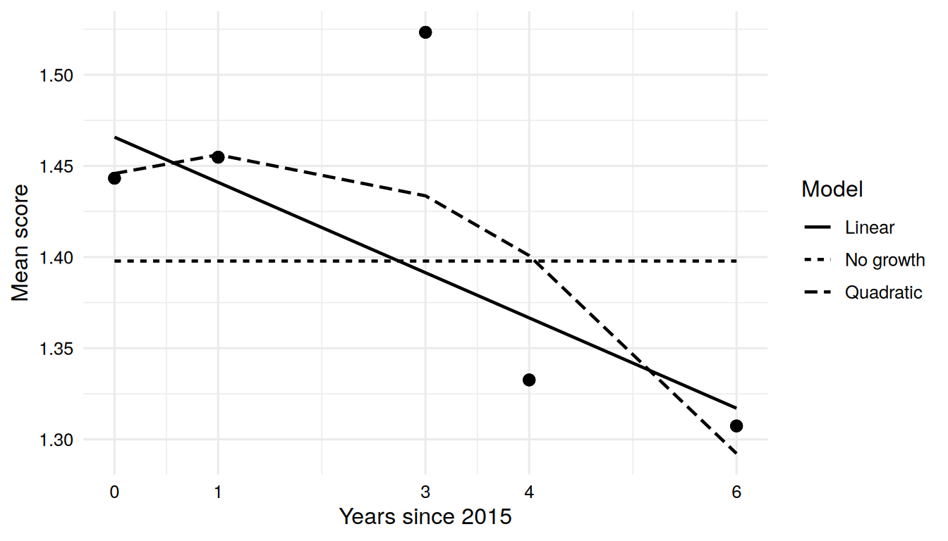
We can also compare what the model implies with what we observe. The model-implied means are a straight line from 1.466 in 2015 down to 1.317 in 2021. The observed means of the 321 participants in the analysis go up from 1.443 at the first wave to 1.523 at the third wave and then fall to 1.307 at the fifth wave (see Figure 2.6 below). A straight line cannot reproduce a rise followed by a fall, and this is one reason to expect that the linear model fits poorly.
2.4.7 What changed compared with the previous model
Compared with the no growth model, we added three parameters: the mean of the slope, the variance of the slope and the covariance between the intercept and the slope. The degrees of freedom went from 13 to 10. The chi-square dropped from 186.433 to 75.244, the CFI rose from .607 to .852 and the RMSEA fell from .204 to .143. The mean of the intercept changed from 1.398 to 1.466 because it now refers to time 0 and not to the average across waves.
2.4.8 What this model answers and what it cannot tell
The linear model answers whether there is an average linear change and whether participants differ in it. The estimates suggest both. It cannot tell whether the change is really linear, because a model that fits poorly is not a good description of the shape. It also says nothing about why participants differ in their slopes. That is the task of the models with covariates in later chapters.
2.5 Model 3: the quadratic growth model
2.5.1 The idea in plain language
A third growth factor allows the rate of change to speed up or slow down. The quadratic factor is a curvature term. With a negative mean quadratic factor, the curve bends downward, which means that an upward trend flattens and turns, or a downward trend becomes steeper. The shape of the curve in the data comes from the combination of all three factors. Several other nonlinear shapes exist, and Grimm et al. (2011) give an overview of them in developmental research.
2.5.2 A concrete example
The observed wave means rise a little and then fall. This is the kind of pattern that a curved trajectory can describe. We therefore ask whether adding the quadratic factor improves the data to model correspondence enough to justify the extra parameters.
where the quadratic loadings are the squares of the slope loadings, that is 0, 1, 9, 16 and 36 (Bollen & Curran, 2006). The quadratic factor \(\eta_{2i}\) has a mean and a variance, and covariances with the intercept and with the slope. This adds four parameters to the linear model. Figure 2.5 shows the diagram. Notice that when a quadratic factor is in the model, the meaning of the slope factor changes. It is no longer the average rate of change over the whole period. It is the rate of change at time 0, that is in 2015.
Figure 2.5: The quadratic growth model as a path diagram. The intercept factor (I) has loadings of 1.0. The slope factor (S) has loadings of 0.0, 1.0, 3.0, 4.0 and 6.0. The quadratic factor (Q) has loadings of 0.0, 1.0, 9.0, 16.0 and 36.0. Three curved arrows connect the three growth factors. Source: workshop slides (Anyan, 2023).
lavaan 0.6.17 ended normally after 79 iterations

  Estimator                                         ML
  Optimization method                           NLMINB
  Number of model parameters                        14

                                                  Used       Total
  Number of observations                           321         442

Model Test User Model:

  Test statistic                                46.671
  Degrees of freedom                                 6
  P-value (Chi-square)                           0.000

Model Test Baseline Model:

  Test statistic                               451.170
  Degrees of freedom                                10
  P-value                                        0.000

User Model versus Baseline Model:

  Comparative Fit Index (CFI)                    0.908
  Tucker-Lewis Index (TLI)                       0.846

Loglikelihood and Information Criteria:

  Loglikelihood user model (H0)               -744.754
  Loglikelihood unrestricted model (H1)       -721.418

  Akaike (AIC)                                1517.507
  Bayesian (BIC)                              1570.308
  Sample-size adjusted Bayesian (SABIC)       1525.902

Root Mean Square Error of Approximation:

  RMSEA                                          0.145
  90 Percent confidence interval - lower         0.108
  90 Percent confidence interval - upper         0.185
  P-value H_0: RMSEA <= 0.050                    0.000
  P-value H_0: RMSEA >= 0.080                    0.998

Standardized Root Mean Square Residual:

  SRMR                                           0.074

Parameter Estimates:

  Standard errors                             Standard
  Information                                 Expected
  Information saturated (h1) model          Structured

Latent Variables:
                   Estimate  Std.Err  z-value  P(>|z|)
  i =~
    lone1             1.000
    lone2             1.000
    lone3             1.000
    lone4             1.000
    lone5             1.000
  s =~
    lone1             0.000
    lone2             1.000
    lone3             3.000
    lone4             4.000
    lone5             6.000
  q =~
    lone1             0.000
    lone2             1.000
    lone3             9.000
    lone4            16.000
    lone5            36.000

Covariances:
                   Estimate  Std.Err  z-value  P(>|z|)
  i ~~
    s                -0.020    0.009   -2.179    0.029
    q                 0.000    0.001    0.265    0.791
  s ~~
    q                -0.002    0.001   -1.792    0.073

Intercepts:
                   Estimate  Std.Err  z-value  P(>|z|)
    i                 1.446    0.024   60.828    0.000
    s                 0.017    0.014    1.284    0.199
    q                -0.007    0.002   -3.384    0.001

Variances:
                   Estimate  Std.Err  z-value  P(>|z|)
   .lone1             0.037    0.014    2.584    0.010
   .lone2             0.118    0.012    9.942    0.000
   .lone3             0.144    0.014   10.115    0.000
   .lone4             0.099    0.011    8.672    0.000
   .lone5             0.099    0.027    3.684    0.000
    i                 0.148    0.019    7.974    0.000
    s                 0.018    0.007    2.697    0.007
    q                 0.000    0.000    0.959    0.337
A typing mistake on the workshop slide
The workshop slide with the results of the quadratic model reports an intercept of 1.466. The correct value is 1.446, as the lavaan output above shows. The value on the slide is a typing mistake. We do not show that slide here, and all numbers for the quadratic model in this chapter come from the R output.
2.5.5 The warning about the latent covariance matrix
Before reading any estimate, look at the warning that lavaan printed after the model was fitted. It says that the covariance matrix of latent variables is not positive definite. This warning means that the estimated variances and covariances of the three growth factors do not form a valid covariance matrix. A valid covariance matrix cannot produce negative variances or correlations larger than 1 in absolute value. We can check what happened with the estimated covariance matrix of the latent variables.
Code
# Addition, not part of the workshop: inspect the latent covariance matrixlavInspect(fit_quadratic, "cov.lv")
       i      s      q
i  0.148
s -0.020  0.018
q  0.000 -0.002  0.000
Code
eigen(lavInspect(fit_quadratic, "cov.lv"))$values
[1] 1.509989e-01 1.500993e-02 -3.256461e-05
Code
cov2cor(lavInspect(fit_quadratic, "cov.lv"))
       i      s      q
i  1.000
s -0.396  1.000
q  0.067 -1.028  1.000
The smallest eigenvalue is slightly negative (about -0.00003). A positive definite matrix has only positive eigenvalues. The variance of the quadratic factor is 0.000 when rounded to three decimals. Its unrounded value is 0.000169 and its standard error is 0.000176 (z = 0.959, p = .337), so the variance is poorly determined. The implied correlation between the slope and the quadratic factor is -1.03, which is not possible for a correlation. The variance is positive, and the problem is the correlation above 1. The solution is therefore inadmissible.
A variance this small does not mean that the factor contributes little. The quadratic loading at the fifth wave is 36, so the variance adds 362 × 0.000169 = 0.22 to the variance of the fifth score. That contribution is offset by the negative covariance with the slope factor, which gives the implied correlation of -1.03. The data do not contain enough information to separate the two factors. The mean of the quadratic factor can still be estimated and describes the average curve. Since the model is flagged, the covariances involving the quadratic factor should not be interpreted, and we cannot conclude from these estimates that participants do not differ in their curvature.
A researcher can fix the variance of the quadratic factor to zero, together with its covariances. The factor then becomes a fixed effect: the average curve bends, and everyone is assumed to share the same curvature. Alternatively, the quadratic factor can be dropped and the linear model kept, or more information can be obtained, for example more participants or more waves. We try the first option below, as an addition to the workshop.
Code
# Addition, not part of the workshop: variance of q (and its covariances) fixed to zeroquadratic_fixed <-paste(quadratic, ' q ~~ 0*q i ~~ 0*q s ~~ 0*q')fit_quadratic_fixed <-growth(quadratic_fixed, data = data)round(fitMeasures(fit_quadratic_fixed, c("chisq", "df", "cfi", "tli", "rmsea", "srmr", "aic", "bic")), 3)
This model runs without the warning. It has 9 degrees of freedom, a chi-square of 63.907, CFI = .876 and RMSEA = .138. It fits better than the linear model but not as well as the quadratic model with the free variance. The chi-square difference with the full quadratic model is 17.236 on 3 degrees of freedom (p < .001). Fixing the variance to zero worsens the fit. Because the test is at a boundary, the p-value is approximate (Self & Liang, 1987). The BIC of the two models is almost identical (1570.2 and 1570.3). The mean of the quadratic factor is -0.007 in the fixed version, the same value as in the free version.
2.5.6 Understanding the output
The chi-square of the quadratic model is 46.671 on 6 degrees of freedom (p < .001), the CFI is .908, the TLI is .846, the RMSEA is .145 (90% CI .108 to .185) and the SRMR is .074. The model has 14 free parameters and uses 321 participants. Compared with the linear model, the CFI and the SRMR are better, the TLI is slightly worse, and the RMSEA is essentially the same. None of the indices reaches the usual guidelines for good fit.
The growth factor means are 1.446 for the intercept (SE = 0.024), 0.017 for the slope (SE = 0.014, p = .199) and -0.007 for the quadratic factor (SE = 0.002, p = .001). The intercept variance is 0.148, the slope variance is 0.018 (p = .007) and the quadratic variance is 0.000 (p = .337). The covariance between the intercept and the slope is -0.020 (p = .029). The covariance between the intercept and the quadratic factor is 0.000 (p = .791) and between the slope and the quadratic factor it is -0.002 (p = .073). The last two covariances are attached to the quadratic variance, and for the reasons given above we do not interpret them.
2.5.7 Interpretation
The mean of the quadratic factor is negative and clearly different from zero, which suggests that the average curve bends downward. The mean of the slope is now small and not different from zero. This does not contradict the linear model, in which the slope was -0.025. The two slopes answer different questions. In the linear model the slope is the average rate of change over the period. In the quadratic model it is the rate of change at 2015, and the later rate depends on the curvature. If we take the estimated means at face value, the model-implied average score rises very slightly from 1.446 in 2015 to 1.456 in 2016, reaches its maximum about 1.22 years after 2015, and then falls to 1.292 in 2021. The fall from 2016 to 2021 is 0.164 units, which is about 0.43 of the standard deviation of the intercept factor (0.38). Since the mean of the slope is not distinguishable from zero, we should not make much of the exact turning point.
Thus, the slope variance means something different in each model. It is 0.018 in the quadratic model and 0.003 in the linear model. In the quadratic model it describes how much participants differ in their rate of change at time 0. It is tied to the quadratic factor: with the quadratic variance and its covariances fixed to zero, the slope variance is 0.003. It is therefore not comparable with the slope variance from the linear model.
Figure 2.6 shows the observed means of the participants in the analysis next to the model-implied means of the three models.
Figure 2.6: Observed wave means of the 321 participants in the analysis (points) and the model-implied means of the no growth, linear and quadratic models (lines). The horizontal axis is time in years since 2015.
Code
knitr::kable(round(means_tab, 3), row.names =FALSE, caption ="Observed and model-implied means at the five waves.")
Observed and model-implied means at the five waves.
time
Observed
No growth
Linear
Quadratic
0
1.443
1.398
1.466
1.446
1
1.455
1.398
1.441
1.456
3
1.523
1.398
1.391
1.434
4
1.333
1.398
1.367
1.401
6
1.307
1.398
1.317
1.292
The quadratic curve is closer to the observed means than the straight line at the first three waves, but the straight line is closer at the fourth and fifth waves. At the fourth wave the quadratic curve misses by 0.068 and the straight line by 0.034. Both curves underestimate the third wave: the observed mean there is 1.523, the quadratic model implies 1.434 and the linear model implies 1.391. A quadratic curve can bend only once, and the observed means seem to go up, then down, and the drop between the third and the fourth wave is sharper than a smooth curve of this kind allows. This helps to explain why the fit remains poor.
2.5.8 What changed compared with the previous model
Compared with the linear model, we added the quadratic factor with its mean, its variance and two covariances. The degrees of freedom went from 10 to 6. The chi-square went from 75.244 to 46.671, the CFI from .852 to .908 and the SRMR from .097 to .074. The slope mean changed sign and is no longer different from zero, and the slope variance rose from 0.003 to 0.018, because the slope now refers to the rate of change at time 0. The model also produced the warning discussed above, which the linear model did not.
2.5.9 What this model answers and what it cannot tell
The quadratic model asks whether the average trajectory is curved. The estimate suggests that it is, with a negative curvature. It cannot tell whether participants differ in their curvature, because the variance of the quadratic factor is not reliably estimated. It also cannot say that a quadratic curve is the right shape. The fit remains poor and the third wave is still not reproduced.
2.6 Comparing the models
The three models are nested. The no growth model is the linear model with the slope mean, the slope variance and the covariance fixed to zero. The linear model is the quadratic model with the quadratic mean, variance and the two covariances fixed to zero. A nested pair can be compared with a chi-square difference test (Bentler & Bonett, 1980). The reduced model has fewer free parameters and the more complex model has more. If the more complex model fits significantly better, the reduced model is rejected. The AIC (Akaike, 1974) and the BIC (Schwarz, 1978) also compare the models. Both penalize the number of parameters, and lower values are preferred.
In lavaan the comparison is done with anova(). The output lists the models with the more constrained one last.
The first test compares the no growth model with the linear model. The chi-square difference is 111.19 on 3 degrees of freedom, with p < .001. In words, the no growth model is rejected, so the linear model fits better. The difference of 3 degrees of freedom is the three parameters added by the slope factor. The AIC is lower for the linear model (1538.1 against 1643.3) and so is the BIC (1575.8 against 1669.7).
The second test compares the linear model with the quadratic model. The chi-square difference is 28.573 on 4 degrees of freedom, with p < .001. The linear model is rejected, so the quadratic model fits better. The AIC is lower for the quadratic model (1517.5 against 1538.1) and so is the BIC (1570.3 against 1575.8), although the difference in BIC is small.
Both tests set a variance to zero in the reduced model, the slope variance in the first and the quadratic variance in the second. A variance of zero lies on the boundary of the parameter space, so the reference distribution of the chi-square difference is not an exact chi-square distribution and the p-values are only approximate (Self & Liang, 1987). The scores are also skewed (Chapter 1), so the standard ML chi-square is itself uncertain. For robust estimators a scaled difference test has to be used (Satorra & Bentler, 2001), and the comparisons above use the standard ML chi-square.
Compare models that fit, and read the comparison with the fit
A chi-square difference test only compares two models with each other. When both models fit poorly, a significant difference means that one is less bad than the other. The CFI of the quadratic model is .908 and the RMSEA is .145. Only models with acceptable fit should be compared for substantive conclusions. Always report the fit of each model next to the comparison, and avoid substantive conclusions about the shape of change until a model with acceptable fit is found.
Fit of the three models (321 participants).
npar
chisq
df
cfi
tli
rmsea
srmr
aic
bic
No growth
7
186.433
13
0.607
0.698
0.204
0.172
1643.269
1669.669
Linear
10
75.244
10
0.852
0.852
0.143
0.097
1538.080
1575.795
Quadratic
14
46.671
6
0.908
0.846
0.145
0.074
1517.507
1570.308
2.7 Sensitivity to the missing data handling
This section is an addition to the workshop. The models above use listwise deletion, so 121 of the 442 rows are not used. Chapter 1 explains listwise deletion and full information maximum likelihood (FIML) and runs this check for the linear model. Here we refit the linear model with FIML, which uses all the available scores of each participant.
Code
# Addition, not part of the workshop: same linear model, FIML instead of listwise deletionfit_linear_fiml <-growth(linear, data = data, missing ="fiml")lavInspect(fit_linear_fiml, "ntotal")
FIML uses 436 participants. The other six rows have no loneliness score at any of the five waves, and lavaan leaves them out. The estimates of the growth factor means change little: the intercept is 1.490 under FIML and 1.466 under listwise deletion, and the slope is -0.027 under FIML and -0.025 under listwise deletion. The variances are somewhat larger under FIML. The conclusions about the direction of the average change and the presence of between-person differences stay the same. The fit statistics of the two runs are not comparable because the numbers of participants differ.
2.8 Researcher’s perspective
The time scores 0, 1, 3, 4 and 6 follow the real spacing of the waves. Equal spacing, such as 0, 1, 2, 3, 4, would give a different slope estimate, -0.037 per step against -0.025 per year, but essentially the same fit (chi-square 75.355 against 75.244, CFI .852 in both). The fit therefore does not show whether the time scores are right, and they have to be chosen from the spacing of the waves.
Models are compared by starting with the reduced model, adding one feature at a time, and using the chi-square difference test together with AIC and BIC. The fit of each model by itself is then examined. In our case no model reaches acceptable fit, and the comparisons are therefore best described as showing that the data favor more flexibility in the mean trajectory than a flat line or a straight line. They do not show that the quadratic model is correct.
A warning about a covariance matrix that is not positive definite is information about the model and the data. Report it, check the latent covariance matrix, and say which choice you made afterwards: keep the model and refrain from interpreting the affected parameters, fix the variance to zero, or drop the factor. Do not change the model until the warning disappears and then report only the final version.
State the number of participants used and the way missing data were handled, and report a check with FIML when listwise deletion removes many rows.
In the next chapter we keep the same data and ask whether a model with two linear pieces fits the loneliness scores better than one smooth curve, since the observed means appear to rise and then fall (see Chapter 3).
Akaike, H. (1974). A new look at the statistical model identification. IEEE Transactions on Automatic Control, 19(6), 716–723. https://doi.org/10.1109/TAC.1974.1100705
Anyan, F. (2023). Longitudinal data analysis using Mplus and R. Workshop slides.
Bentler, P. M., & Bonett, D. G. (1980). Significance tests and goodness of fit in the analysis of covariance structures. Psychological Bulletin, 88(3), 588–606. https://doi.org/10.1037/0033-2909.88.3.588
Bollen, K. A., & Curran, P. J. (2006). Latent curve models: A structural equation perspective. Wiley.
Hu, L., & Bentler, P. M. (1999). Cutoff criteria for fit indexes in covariance structure analysis: Conventional criteria versus new alternatives. Structural Equation Modeling: A Multidisciplinary Journal, 6(1), 1–55. https://doi.org/10.1080/10705519909540118
Preacher, K. J., Wichman, A. L., MacCallum, R. C., & Briggs, N. E. (2008). Latent growth curve modeling. Sage.
Satorra, A., & Bentler, P. M. (2001). A scaled difference chi-square test statistic for moment structure analysis. Psychometrika, 66(4), 507–514. https://doi.org/10.1007/BF02296192
Schwarz, G. (1978). Estimating the dimension of a model. The Annals of Statistics, 6(2), 461–464.
Self, S. G., & Liang, K.-Y. (1987). Asymptotic properties of maximum likelihood estimators and likelihood ratio tests under nonstandard conditions. Journal of the American Statistical Association, 82(398), 605–610. https://doi.org/10.1080/01621459.1987.10478472
Source Code
# No growth, linear and quadratic growth models {#sec-basic}```{r}#| label: setup#| include: falselibrary(lavaan)library(dplyr)library(tidyr)library(ggplot2)library(psych)data <-read.csv("data/data.csv", fileEncoding ="UTF-8-BOM")theme_set(theme_minimal(base_size =12) +theme(plot.title =element_text(face ="bold", color ="black"),axis.title =element_text(color ="black"),axis.text =element_text(color ="black"),strip.text =element_text(color ="black"),legend.text =element_text(color ="black")))``````{r}#| label: helpers#| include: falsef3 <-function(x) formatC(x, format ="f", digits =3)f2 <-function(x) formatC(x, format ="f", digits =2)lone <-paste0("lone", 1:5)n_used <-sum(complete.cases(data[, lone]))nz <-function(x, d =3) sub("^(-?)0\\.", "\\1.", formatC(x, format ="f", digits = d))fx <-function(fit, m, d =3) formatC(unname(fitMeasures(fit, m)), format ="f", digits = d)fxn <-function(fit, m) nz(unname(fitMeasures(fit, m)))pv <-function(fit, l, o, r ="", what ="est") { p <-parameterEstimates(fit) p[p$lhs == l & p$op == o & p$rhs == r, what]}g <-function(fit, l, o, r ="", d =3, what ="est") formatC(pv(fit, l, o, r, what), format ="f", digits = d)rv <-function(fit) sapply(lone, function(v) pv(fit, v, "~~", v))imp <-function(fit) as.numeric(fitted(fit)$mean)obs <-colMeans(data[complete.cases(data[, lone]), lone])```In @sec-prelims we looked at the data before fitting anything: the means and spread of the loneliness scores at each wave, the correlations across waves, the missing data, and the choice of time scores. In this chapter we fit the first three growth models to those five waves. We start with the simplest model, in which nothing changes over time, and then add a *linear growth model* and a *quadratic growth model*. Each model contains the one before it as a special case, which allows us to ask at every step whether the added part is needed.## Why start with simple modelsA growth model is a statement about how the average level of the outcome moves over time and about how much people differ around that average. We start with the simplest model and add one feature at a time, so each addition answers one question.The three models in this chapter answer three questions.1. Is there a stable level of loneliness and do participants differ in that level, with no systematic change over time? (*no growth model*)2. Does the average level change at a constant rate and do participants differ in their rate of change? (*linear growth model*)3. Does the rate of change itself change over the waves? (*quadratic growth model*)The ideas behind these models come from the latent curve framework, in which a growth model is a confirmatory factor model with the loadings tied to time [@meredith1990latent]. The structural equation perspective is treated in full by @bollen2006latent. Introductions with applied examples are given by @duncan2004introduction and @preacher2008latent. We use the same dataset and the same five waves for all three models, so any difference between them is a difference in the model and not in the data.## The data and the time scoresThe dataset has 442 rows. The loneliness scores `lone1` to `lone5` were measured at five waves in 2015, 2016, 2018, 2019 and 2021. The gaps between waves are 1, 2, 1 and 2 years, and we therefore use the time scores 0, 1, 3, 4 and 6, with 2015 as time 0 and one unit equal to one year. The reasons were given in @sec-prelims. In all three models below, the time scores enter the model as fixed factor loadings.In the workshop script `growth()` is called with its default settings, which means listwise deletion. Of the 442 rows, `r n_used` have scores on all five waves, and all three models are estimated on these `r n_used` participants. The output reports this as "Used `r n_used`, Total 442". Listwise deletion, full information maximum likelihood and the missing data assumptions are explained in @sec-prelims. The loneliness scores are also skewed (@sec-prelims), which matters for the chi-square tests of fit and for the comparison of the models below.## Model 1: the no growth model### The idea in plain languageThe *no growth model*, also called the intercept-only model, is the reduced model of this chapter. It says that each participant has a stable true level of loneliness that does not change over the five waves. Participants may differ in that level, and the observed scores at each wave differ from the participant's level only because of measurement error and occasional fluctuation. If this model fitted well, there would be no reason to look for growth.The model has one growth factor, the *intercept factor*. Its mean is the average level across participants and its variance tells us how much participants differ in their level. Each wave has its own residual variance.### A concrete exampleFor the loneliness scores, the no growth model says that a participant who scores high at the first wave has a high true level at all later waves, and that the mean of the five wave means is a sufficient description of the average. We know from the descriptive output that the wave means are not identical, so the model is likely too simple. We fit it anyway because it is the baseline against which every other model in the chapter is compared.### The formal modelFor participant $i$ at wave $t$, the observed score is$$y_{ti} = \eta_{0i} + \varepsilon_{ti},$$where $\eta_{0i}$ is the intercept factor and $\varepsilon_{ti}$ is the residual with variance $\theta_t$ [@bollen2006latent]. The intercept factor has a mean $\alpha_0$ and a variance $\psi_{00}$, so that $\eta_{0i} = \alpha_0 + \zeta_{0i}$. All five loadings of the intercept factor are fixed to 1. @fig-nogrowth-diagram shows the path diagram from the workshop.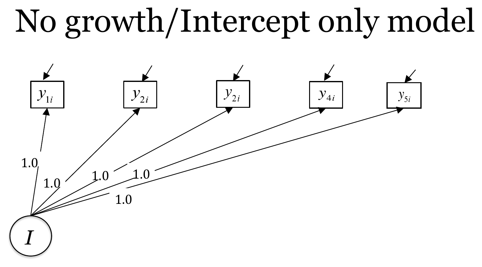{#fig-nogrowth-diagram fig-alt="Path diagram of the no growth model with one intercept factor and five observed variables" width="80%"}### R implementationIn the workshop syntax the loadings of the intercept factor are fixed to 1 and nothing else is specified. The growth factor mean and the variances are added by `growth()`.```{r}#| label: fit-nogrowthnogrowth <-' i =~ 1*lone1 + 1*lone2 + 1*lone3 + 1*lone4 + 1*lone5'fit_nogrowth <-growth(nogrowth, data = data)summary(fit_nogrowth, fit.measures =TRUE)```### Understanding the outputThe header shows that `r n_used` of 442 rows were used. The model has `r fx(fit_nogrowth, "npar", 0)` free parameters: the mean and variance of the intercept factor and the five residual variances. The five observed means, five variances and ten covariances give 20 pieces of information, which leaves `r fx(fit_nogrowth, "df", 0)` degrees of freedom. The chi-square test is `r fx(fit_nogrowth, "chisq")` on `r fx(fit_nogrowth, "df", 0)` degrees of freedom with *p* < .001, which means that the model-implied means and covariances differ from the observed ones by more than sampling error would explain. The CFI is `r fxn(fit_nogrowth, "cfi")`, the TLI is `r fxn(fit_nogrowth, "tli")`, the RMSEA is `r fxn(fit_nogrowth, "rmsea")` (90% CI `r fxn(fit_nogrowth, "rmsea.ci.lower")` to `r fxn(fit_nogrowth, "rmsea.ci.upper")`) and the SRMR is `r fxn(fit_nogrowth, "srmr")`. Guidelines for these indices are discussed in @hu1999cutoff. They are not fixed rules, but values of this size are far from the usual cut-offs. The no growth model does not describe these data well.The intercept mean is `r g(fit_nogrowth, "i", "~1")` and the variance of the intercept factor is `r g(fit_nogrowth, "i", "~~", "i")`, both with *p* < .001. The residual variances range from `r f3(min(rv(fit_nogrowth)))` to `r f3(max(rv(fit_nogrowth)))`. @fig-nogrowth-results shows the same model with the results as they were reported in the workshop. These numbers were estimated in Mplus. The R output above is the one used in this chapter, and the two agree for the fit statistics, the intercept mean and the intercept variance. The slide prints the largest residual variance as 1.167. This is a typing mistake in the workshop slide. The correct value is `r f3(max(rv(fit_nogrowth)))`, as the R output shows, and we use that value throughout.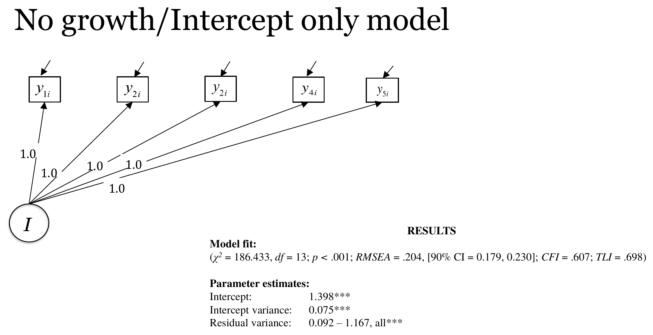{#fig-nogrowth-results fig-alt="No growth model path diagram with model fit statistics and parameter estimates" width="90%"}### InterpretationParticipants are estimated to have an average level of `r g(fit_nogrowth, "i", "~1")` on the original score metric. The intercept variance of `r g(fit_nogrowth, "i", "~~", "i")` is clearly different from zero, so there are between-person differences in level. These statements describe this dataset and this model. Since the fit is poor, we do not give weight to the exact size of the estimates. The poor fit tells us that a single stable level for each participant is not enough to reproduce the pattern of means and covariances across the five waves.### What this model answers and what it cannot tellThe no growth model answers the question of whether participants differ in a stable level. It cannot say anything about change, because change is excluded by design. Its main use is as the reference point for the next model.## Model 2: the linear growth model### The idea in plain languageIf scores change over time at a constant rate, a second growth factor is needed. The *slope factor* describes the rate of change per time unit. Participants may have different starting levels and different rates of change, so both growth factors have a variance. The intercept and the slope may also be related, and this relation is estimated as a covariance.### A concrete exampleThe linear model describes each participant by a straight line over the years 2015 to 2021. The intercept factor is the expected score in 2015, which is time 0. The slope factor is the expected change in score per year. The model asks whether the average slope differs from zero and whether participants differ in their slopes.### The formal model$$y_{ti} = \eta_{0i} + \lambda_t \, \eta_{1i} + \varepsilon_{ti}, \qquad \lambda_t = 0, 1, 3, 4, 6,$$with $\eta_{0i} = \alpha_0 + \zeta_{0i}$ and $\eta_{1i} = \alpha_1 + \zeta_{1i}$ [@bollen2006latent]. The model has two means ($\alpha_0$, $\alpha_1$), two variances ($\psi_{00}$, $\psi_{11}$), one covariance ($\psi_{01}$) and the five residual variances. @fig-linear-diagram shows the diagram.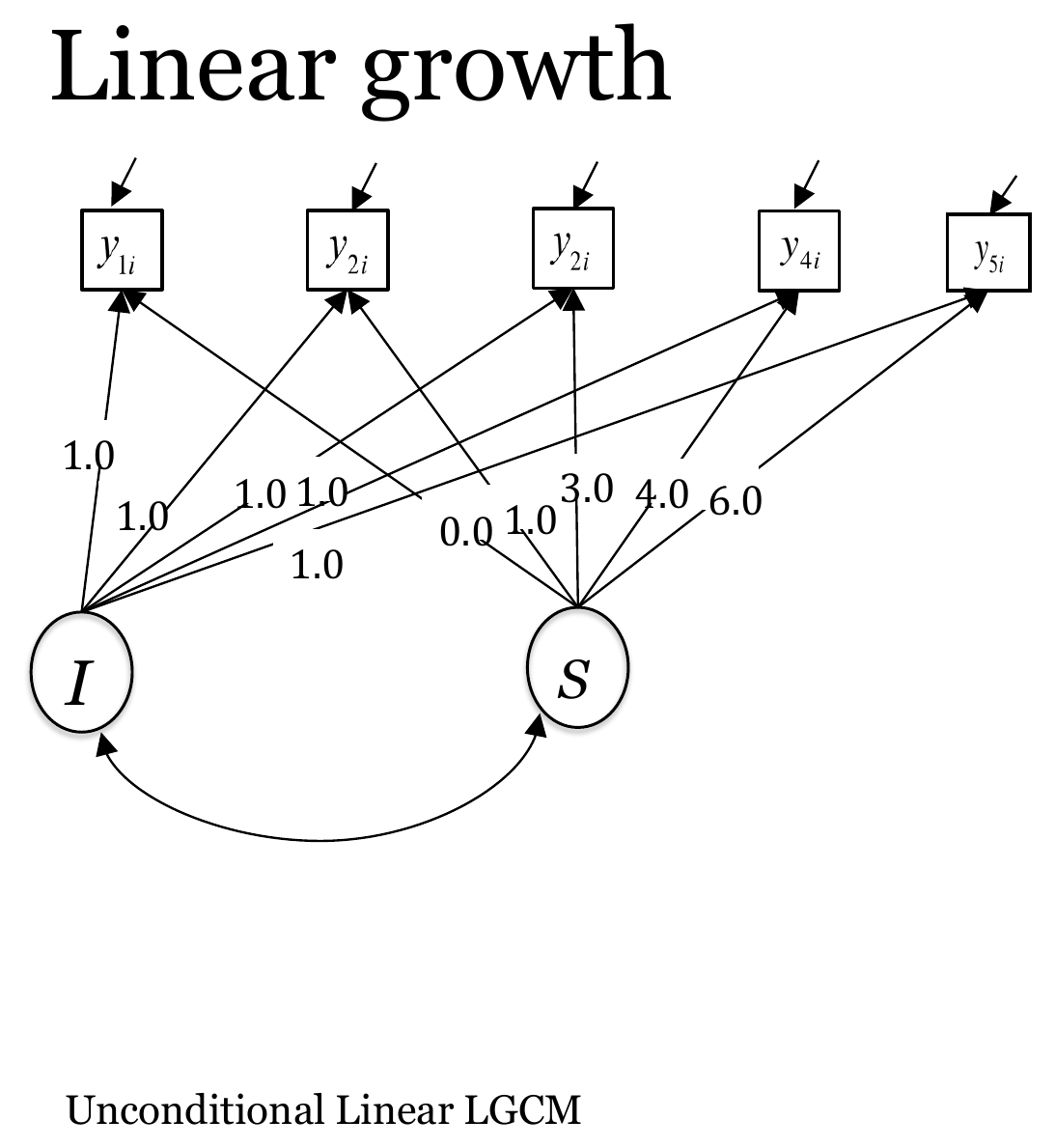{#fig-linear-diagram fig-alt="Path diagram of the linear growth model with an intercept factor, a slope factor and their covariance" width="60%"}### R implementationThe only change in the syntax is the second line, which adds the slope factor with the time scores as loadings.```{r}#| label: fit-linearlinear <-' i =~ 1*lone1 + 1*lone2 + 1*lone3 + 1*lone4 + 1*lone5 s =~ 0*lone1 + 1*lone2 + 3*lone3 + 4*lone4 + 6*lone5'fit_linear <-growth(linear, data = data)summary(fit_linear, fit.measures =TRUE)```### Understanding the outputThe linear model has `r fx(fit_linear, "npar", 0)` free parameters and `r fx(fit_linear, "df", 0)` degrees of freedom. The chi-square is `r fx(fit_linear, "chisq")` with *p* < .001. The CFI is `r fxn(fit_linear, "cfi")`, the TLI is `r fxn(fit_linear, "tli")`, the RMSEA is `r fxn(fit_linear, "rmsea")` (90% CI `r fxn(fit_linear, "rmsea.ci.lower")` to `r fxn(fit_linear, "rmsea.ci.upper")`) and the SRMR is `r fxn(fit_linear, "srmr")`. The fit is clearly better than that of the no growth model, but it still does not reach the usual guidelines. The number of participants used is again `r n_used`.The estimates show a mean intercept of `r g(fit_linear, "i", "~1")` (SE = `r g(fit_linear, "i", "~1", what = "se")`) and a mean slope of `r g(fit_linear, "s", "~1")` (SE = `r g(fit_linear, "s", "~1", what = "se")`, *p* < .001). The variance of the intercept factor is `r g(fit_linear, "i", "~~", "i")` and the variance of the slope factor is `r g(fit_linear, "s", "~~", "s")`, both with *p* < .001. The covariance between the intercept and the slope is `r g(fit_linear, "i", "~~", "s")` (*p* < .001). Notice that the residual variances are freely estimated and differ across waves, from `r f3(rv(fit_linear)["lone5"])` at the fifth wave to `r f3(rv(fit_linear)["lone3"])` at the third wave. @fig-linear-results shows the Mplus results from the workshop, which agree with the R output.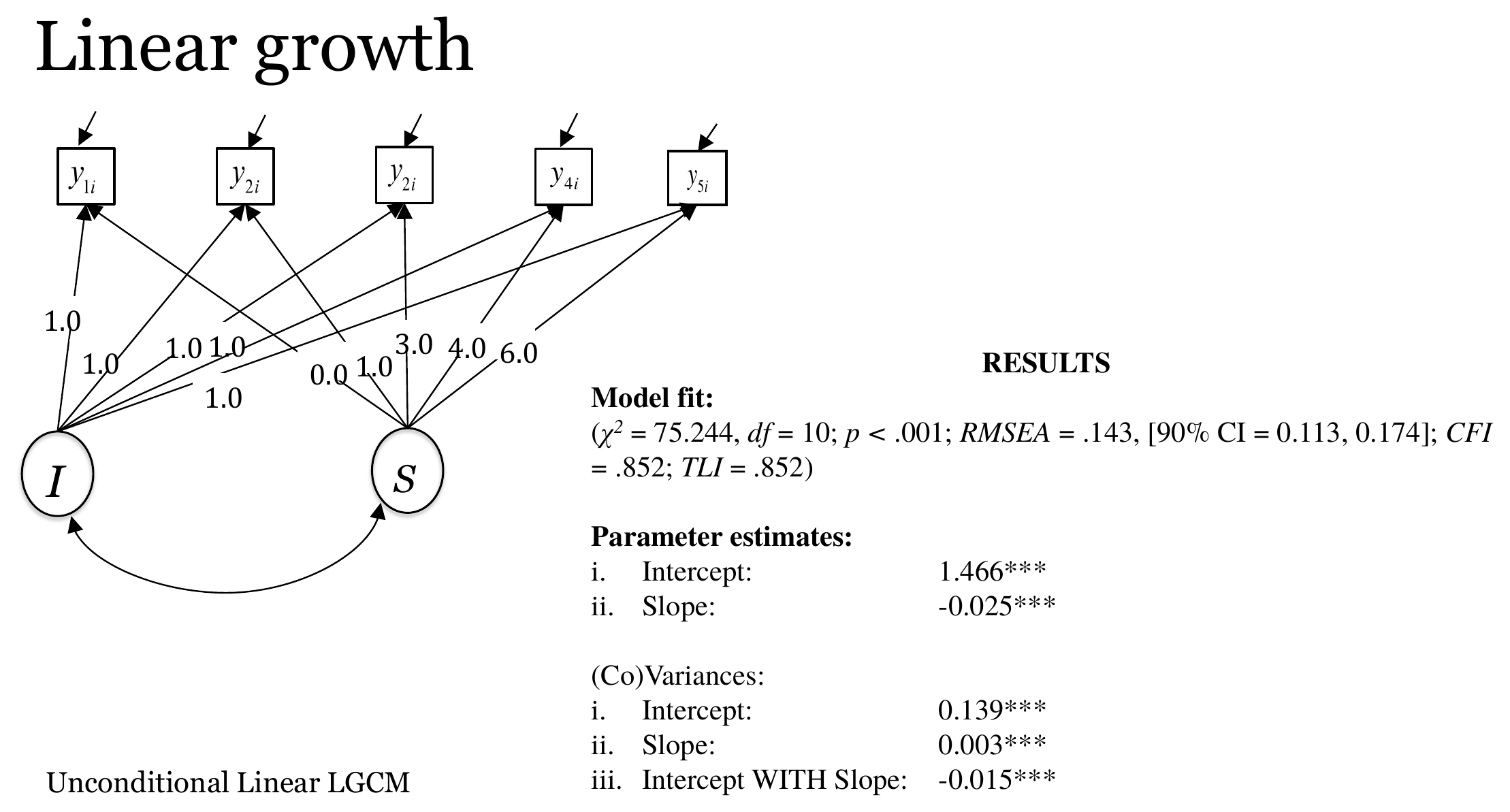{#fig-linear-results fig-alt="Linear growth model path diagram with model fit statistics and estimates for means, variances and covariance" width="90%"}### Interpretation```{r}#| label: linear-interp-values#| include: falseslope_lin <-pv(fit_linear, "s", "~1")sd_i_lin <-sqrt(pv(fit_linear, "i", "~~", "i"))sd_s_lin <-sqrt(pv(fit_linear, "s", "~~", "s"))```The average score in 2015 is estimated to be `r g(fit_linear, "i", "~1")`, and the average change is `r g(fit_linear, "s", "~1")` units per year. Over the six years from 2015 to 2021 this amounts to a decrease of about `r f2(abs(6 * slope_lin))` units on average. The standard deviation of the intercept factor is `r f2(sd_i_lin)`, so the average decrease is about `r f2(abs(6 * slope_lin) / sd_i_lin)` of that standard deviation. The slope variance of `r g(fit_linear, "s", "~~", "s")` corresponds to a standard deviation of about `r f3(sd_s_lin)`. If the slopes are roughly normally distributed, about 95% of the participants would have yearly slopes between `r f2(slope_lin - 2 * sd_s_lin)` and `r f2(slope_lin + 2 * sd_s_lin)`. That is to say, the average slope is negative, but the spread is consistent with a positive slope for some participants.The correlation between the intercept and the slope is `r f2(cov2cor(lavInspect(fit_linear, "cov.lv"))[2, 1])`. Participants with a higher level in 2015 tend to have a more negative slope. Two cautions apply. First, the lowest observed score is 1 at every wave and most values are close to it, so a participant who starts near the bottom has little room to decline. A negative association between the starting level and the change could partly reflect this. Second, the slope variance is small in absolute terms, and the correlation is therefore estimated from a factor with little variance to work with.We can also compare what the model implies with what we observe. The model-implied means are a straight line from `r f3(imp(fit_linear)[1])` in 2015 down to `r f3(imp(fit_linear)[5])` in 2021. The observed means of the `r n_used` participants in the analysis go up from `r f3(obs[1])` at the first wave to `r f3(obs[3])` at the third wave and then fall to `r f3(obs[5])` at the fifth wave (see @fig-means below). A straight line cannot reproduce a rise followed by a fall, and this is one reason to expect that the linear model fits poorly.### What changed compared with the previous modelCompared with the no growth model, we added three parameters: the mean of the slope, the variance of the slope and the covariance between the intercept and the slope. The degrees of freedom went from `r fx(fit_nogrowth, "df", 0)` to `r fx(fit_linear, "df", 0)`. The chi-square dropped from `r fx(fit_nogrowth, "chisq")` to `r fx(fit_linear, "chisq")`, the CFI rose from `r fxn(fit_nogrowth, "cfi")` to `r fxn(fit_linear, "cfi")` and the RMSEA fell from `r fxn(fit_nogrowth, "rmsea")` to `r fxn(fit_linear, "rmsea")`. The mean of the intercept changed from `r g(fit_nogrowth, "i", "~1")` to `r g(fit_linear, "i", "~1")` because it now refers to time 0 and not to the average across waves.### What this model answers and what it cannot tellThe linear model answers whether there is an average linear change and whether participants differ in it. The estimates suggest both. It cannot tell whether the change is really linear, because a model that fits poorly is not a good description of the shape. It also says nothing about why participants differ in their slopes. That is the task of the models with covariates in later chapters.## Model 3: the quadratic growth model### The idea in plain languageA third growth factor allows the rate of change to speed up or slow down. The *quadratic factor* is a curvature term. With a negative mean quadratic factor, the curve bends downward, which means that an upward trend flattens and turns, or a downward trend becomes steeper. The shape of the curve in the data comes from the combination of all three factors. Several other nonlinear shapes exist, and @grimm2011nonlinear give an overview of them in developmental research.### A concrete exampleThe observed wave means rise a little and then fall. This is the kind of pattern that a curved trajectory can describe. We therefore ask whether adding the quadratic factor improves the data to model correspondence enough to justify the extra parameters.### The formal model$$y_{ti} = \eta_{0i} + \lambda_t \, \eta_{1i} + \lambda_t^2 \, \eta_{2i} + \varepsilon_{ti},$$where the quadratic loadings are the squares of the slope loadings, that is 0, 1, 9, 16 and 36 [@bollen2006latent]. The quadratic factor $\eta_{2i}$ has a mean and a variance, and covariances with the intercept and with the slope. This adds four parameters to the linear model. @fig-quadratic-diagram shows the diagram. Notice that when a quadratic factor is in the model, the meaning of the slope factor changes. It is no longer the average rate of change over the whole period. It is the rate of change at time 0, that is in 2015.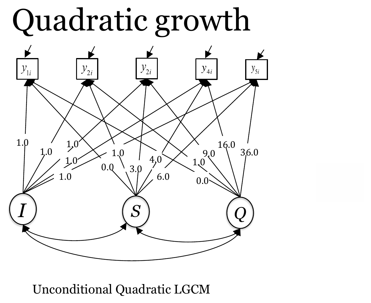{#fig-quadratic-diagram fig-alt="Path diagram of the quadratic growth model with intercept, slope and quadratic factors and three covariances" width="70%"}### R implementation```{r}#| label: fit-quadraticquadratic <-' i =~ 1*lone1 + 1*lone2 + 1*lone3 + 1*lone4 + 1*lone5 s =~ 0*lone1 + 1*lone2 + 3*lone3 + 4*lone4 + 6*lone5 q =~ 0*lone1 + 1*lone2 + 9*lone3 + 16*lone4 + 36*lone5'fit_quadratic <-growth(quadratic, data = data)summary(fit_quadratic, fit.measures =TRUE)```::: {.callout-note title="A typing mistake on the workshop slide"}The workshop slide with the results of the quadratic model reports an intercept of 1.466. The correct value is `r g(fit_quadratic, "i", "~1")`, as the lavaan output above shows. The value on the slide is a typing mistake. We do not show that slide here, and all numbers for the quadratic model in this chapter come from the R output.:::### The warning about the latent covariance matrixBefore reading any estimate, look at the warning that lavaan printed after the model was fitted. It says that the covariance matrix of latent variables is not positive definite. This warning means that the estimated variances and covariances of the three growth factors do not form a valid covariance matrix. A valid covariance matrix cannot produce negative variances or correlations larger than 1 in absolute value. We can check what happened with the estimated covariance matrix of the latent variables.```{r}#| label: check-cov-lv# Addition, not part of the workshop: inspect the latent covariance matrixlavInspect(fit_quadratic, "cov.lv")eigen(lavInspect(fit_quadratic, "cov.lv"))$valuescov2cor(lavInspect(fit_quadratic, "cov.lv"))``````{r}#| label: quad-values#| include: falsecl_q <-lavInspect(fit_quadratic, "cov.lv")q_var <- cl_q[3, 3]q_se <-pv(fit_quadratic, "q", "~~", "q", what ="se")q_z <-pv(fit_quadratic, "q", "~~", "q", what ="z")```The smallest eigenvalue is slightly negative (about `r formatC(min(eigen(cl_q)$values), format = "f", digits = 5)`). A positive definite matrix has only positive eigenvalues. The variance of the quadratic factor is 0.000 when rounded to three decimals. Its unrounded value is `r formatC(q_var, format = "f", digits = 6)` and its standard error is `r formatC(q_se, format = "f", digits = 6)` (*z* = `r f3(q_z)`, *p* = .337), so the variance is poorly determined. The implied correlation between the slope and the quadratic factor is `r f2(cov2cor(cl_q)[3, 2])`, which is not possible for a correlation. The variance is positive, and the problem is the correlation above 1. The solution is therefore inadmissible.A variance this small does not mean that the factor contributes little. The quadratic loading at the fifth wave is 36, so the variance adds 36^2^ × `r formatC(q_var, format = "f", digits = 6)` = `r f2(36^2 * q_var)` to the variance of the fifth score. That contribution is offset by the negative covariance with the slope factor, which gives the implied correlation of `r f2(cov2cor(cl_q)[3, 2])`. The data do not contain enough information to separate the two factors. The mean of the quadratic factor can still be estimated and describes the average curve. Since the model is flagged, the covariances involving the quadratic factor should not be interpreted, and we cannot conclude from these estimates that participants do not differ in their curvature.A researcher can fix the variance of the quadratic factor to zero, together with its covariances. The factor then becomes a *fixed effect*: the average curve bends, and everyone is assumed to share the same curvature. Alternatively, the quadratic factor can be dropped and the linear model kept, or more information can be obtained, for example more participants or more waves. We try the first option below, as an addition to the workshop.```{r}#| label: fit-quadratic-fixed# Addition, not part of the workshop: variance of q (and its covariances) fixed to zeroquadratic_fixed <-paste(quadratic, ' q ~~ 0*q i ~~ 0*q s ~~ 0*q')fit_quadratic_fixed <-growth(quadratic_fixed, data = data)round(fitMeasures(fit_quadratic_fixed, c("chisq", "df", "cfi", "tli", "rmsea", "srmr", "aic", "bic")), 3)parameterEstimates(fit_quadratic_fixed) |>filter(op %in%c("~1", "~~"), lhs %in%c("i", "s", "q"), lhs == rhs | op =="~1") |>select(lhs, op, est, se, pvalue)an_fq <-anova(fit_quadratic_fixed, fit_quadratic)an_fq```This model runs without the warning. It has `r fx(fit_quadratic_fixed, "df", 0)` degrees of freedom, a chi-square of `r fx(fit_quadratic_fixed, "chisq")`, CFI = `r fxn(fit_quadratic_fixed, "cfi")` and RMSEA = `r fxn(fit_quadratic_fixed, "rmsea")`. It fits better than the linear model but not as well as the quadratic model with the free variance. The chi-square difference with the full quadratic model is `r f3(an_fq[["Chisq diff"]][2])` on `r an_fq[["Df diff"]][2]` degrees of freedom (*p* < .001). Fixing the variance to zero worsens the fit. Because the test is at a boundary, the *p*-value is approximate [@self1987asymptotic]. The BIC of the two models is almost identical (`r fx(fit_quadratic_fixed, "bic", 1)` and `r fx(fit_quadratic, "bic", 1)`). The mean of the quadratic factor is `r g(fit_quadratic_fixed, "q", "~1")` in the fixed version, the same value as in the free version.### Understanding the outputThe chi-square of the quadratic model is `r fx(fit_quadratic, "chisq")` on `r fx(fit_quadratic, "df", 0)` degrees of freedom (*p* < .001), the CFI is `r fxn(fit_quadratic, "cfi")`, the TLI is `r fxn(fit_quadratic, "tli")`, the RMSEA is `r fxn(fit_quadratic, "rmsea")` (90% CI `r fxn(fit_quadratic, "rmsea.ci.lower")` to `r fxn(fit_quadratic, "rmsea.ci.upper")`) and the SRMR is `r fxn(fit_quadratic, "srmr")`. The model has `r fx(fit_quadratic, "npar", 0)` free parameters and uses `r n_used` participants. Compared with the linear model, the CFI and the SRMR are better, the TLI is slightly worse, and the RMSEA is essentially the same. None of the indices reaches the usual guidelines for good fit.The growth factor means are `r g(fit_quadratic, "i", "~1")` for the intercept (SE = `r g(fit_quadratic, "i", "~1", what = "se")`), `r g(fit_quadratic, "s", "~1")` for the slope (SE = `r g(fit_quadratic, "s", "~1", what = "se")`, *p* = .199) and `r g(fit_quadratic, "q", "~1")` for the quadratic factor (SE = `r g(fit_quadratic, "q", "~1", what = "se")`, *p* = .001). The intercept variance is `r g(fit_quadratic, "i", "~~", "i")`, the slope variance is `r g(fit_quadratic, "s", "~~", "s")` (*p* = .007) and the quadratic variance is `r g(fit_quadratic, "q", "~~", "q")` (*p* = .337). The covariance between the intercept and the slope is `r g(fit_quadratic, "i", "~~", "s")` (*p* = .029). The covariance between the intercept and the quadratic factor is `r g(fit_quadratic, "i", "~~", "q")` (*p* = .791) and between the slope and the quadratic factor it is `r g(fit_quadratic, "s", "~~", "q")` (*p* = .073). The last two covariances are attached to the quadratic variance, and for the reasons given above we do not interpret them.### Interpretation```{r}#| label: quad-interp-values#| include: falsecq <-coef(fit_quadratic)turn_q <--cq["s~1"] / (2* cq["q~1"])sd_i_q <-sqrt(pv(fit_quadratic, "i", "~~", "i"))imp_q <-imp(fit_quadratic)```The mean of the quadratic factor is negative and clearly different from zero, which suggests that the average curve bends downward. The mean of the slope is now small and not different from zero. This does not contradict the linear model, in which the slope was `r g(fit_linear, "s", "~1")`. The two slopes answer different questions. In the linear model the slope is the average rate of change over the period. In the quadratic model it is the rate of change at 2015, and the later rate depends on the curvature. If we take the estimated means at face value, the model-implied average score rises very slightly from `r f3(imp_q[1])` in 2015 to `r f3(imp_q[2])` in 2016, reaches its maximum about `r f2(turn_q)` years after 2015, and then falls to `r f3(imp_q[5])` in 2021. The fall from 2016 to 2021 is `r f3(imp_q[2] - imp_q[5])` units, which is about `r f2((imp_q[2] - imp_q[5]) / sd_i_q)` of the standard deviation of the intercept factor (`r f2(sd_i_q)`). Since the mean of the slope is not distinguishable from zero, we should not make much of the exact turning point.Thus, the slope variance means something different in each model. It is `r g(fit_quadratic, "s", "~~", "s")` in the quadratic model and `r g(fit_linear, "s", "~~", "s")` in the linear model. In the quadratic model it describes how much participants differ in their rate of change at time 0. It is tied to the quadratic factor: with the quadratic variance and its covariances fixed to zero, the slope variance is `r g(fit_quadratic_fixed, "s", "~~", "s")`. It is therefore not comparable with the slope variance from the linear model.@fig-means shows the observed means of the participants in the analysis next to the model-implied means of the three models.```{r}#| label: fig-means#| fig-cap: "Observed wave means of the 321 participants in the analysis (points) and the model-implied means of the no growth, linear and quadratic models (lines). The horizontal axis is time in years since 2015."#| fig-alt: "Line chart of the observed mean loneliness score at the five waves with three model-implied mean curves"#| fig-width: 7#| fig-height: 4means_tab <-data.frame(time =c(0, 1, 3, 4, 6),Observed =colMeans(data[complete.cases(data[, lone]), lone]),`No growth`=as.numeric(fitted(fit_nogrowth)$mean),Linear =as.numeric(fitted(fit_linear)$mean),Quadratic =as.numeric(fitted(fit_quadratic)$mean),check.names =FALSE)means_long <-pivot_longer(means_tab, -c(time, Observed), names_to ="Model", values_to ="Mean")ggplot(means_long, aes(time, Mean, linetype = Model)) +geom_line(linewidth =0.8, color ="black") +geom_point(aes(y = Observed), size =2.5, color ="black") +scale_x_continuous(breaks =c(0, 1, 3, 4, 6)) +labs(x ="Years since 2015", y ="Mean score")``````{r}#| label: means-tableknitr::kable(round(means_tab, 3), row.names =FALSE, caption ="Observed and model-implied means at the five waves.")``````{r}#| label: miss-values#| include: falsemiss_lin <-abs(means_tab$Observed - means_tab$Linear)miss_quad <-abs(means_tab$Observed - means_tab$Quadratic)```The quadratic curve is closer to the observed means than the straight line at the first three waves, but the straight line is closer at the fourth and fifth waves. At the fourth wave the quadratic curve misses by `r f3(miss_quad[4])` and the straight line by `r f3(miss_lin[4])`. Both curves underestimate the third wave: the observed mean there is `r f3(means_tab$Observed[3])`, the quadratic model implies `r f3(means_tab$Quadratic[3])` and the linear model implies `r f3(means_tab$Linear[3])`. A quadratic curve can bend only once, and the observed means seem to go up, then down, and the drop between the third and the fourth wave is sharper than a smooth curve of this kind allows. This helps to explain why the fit remains poor.### What changed compared with the previous modelCompared with the linear model, we added the quadratic factor with its mean, its variance and two covariances. The degrees of freedom went from `r fx(fit_linear, "df", 0)` to `r fx(fit_quadratic, "df", 0)`. The chi-square went from `r fx(fit_linear, "chisq")` to `r fx(fit_quadratic, "chisq")`, the CFI from `r fxn(fit_linear, "cfi")` to `r fxn(fit_quadratic, "cfi")` and the SRMR from `r fxn(fit_linear, "srmr")` to `r fxn(fit_quadratic, "srmr")`. The slope mean changed sign and is no longer different from zero, and the slope variance rose from `r g(fit_linear, "s", "~~", "s")` to `r g(fit_quadratic, "s", "~~", "s")`, because the slope now refers to the rate of change at time 0. The model also produced the warning discussed above, which the linear model did not.### What this model answers and what it cannot tellThe quadratic model asks whether the average trajectory is curved. The estimate suggests that it is, with a negative curvature. It cannot tell whether participants differ in their curvature, because the variance of the quadratic factor is not reliably estimated. It also cannot say that a quadratic curve is the right shape. The fit remains poor and the third wave is still not reproduced.## Comparing the modelsThe three models are *nested*. The no growth model is the linear model with the slope mean, the slope variance and the covariance fixed to zero. The linear model is the quadratic model with the quadratic mean, variance and the two covariances fixed to zero. A nested pair can be compared with a chi-square difference test [@bentler1980significance]. The reduced model has fewer free parameters and the more complex model has more. If the more complex model fits significantly better, the reduced model is rejected. The AIC [@akaike1974new] and the BIC [@schwarz1978estimating] also compare the models. Both penalize the number of parameters, and lower values are preferred.In lavaan the comparison is done with `anova()`. The output lists the models with the more constrained one last.```{r}#| label: model-comparisonsan_nl <-anova(fit_nogrowth, fit_linear)an_lq <-anova(fit_linear, fit_quadratic)an_nlan_lq```The first test compares the no growth model with the linear model. The chi-square difference is `r f2(an_nl[["Chisq diff"]][2])` on `r an_nl[["Df diff"]][2]` degrees of freedom, with *p* < .001. In words, the no growth model is rejected, so the linear model fits better. The difference of 3 degrees of freedom is the three parameters added by the slope factor. The AIC is lower for the linear model (`r fx(fit_linear, "aic", 1)` against `r fx(fit_nogrowth, "aic", 1)`) and so is the BIC (`r fx(fit_linear, "bic", 1)` against `r fx(fit_nogrowth, "bic", 1)`).The second test compares the linear model with the quadratic model. The chi-square difference is `r f3(an_lq[["Chisq diff"]][2])` on `r an_lq[["Df diff"]][2]` degrees of freedom, with *p* < .001. The linear model is rejected, so the quadratic model fits better. The AIC is lower for the quadratic model (`r fx(fit_quadratic, "aic", 1)` against `r fx(fit_linear, "aic", 1)`) and so is the BIC (`r fx(fit_quadratic, "bic", 1)` against `r fx(fit_linear, "bic", 1)`), although the difference in BIC is small.Both tests set a variance to zero in the reduced model, the slope variance in the first and the quadratic variance in the second. A variance of zero lies on the boundary of the parameter space, so the reference distribution of the chi-square difference is not an exact chi-square distribution and the *p*-values are only approximate [@self1987asymptotic]. The scores are also skewed (@sec-prelims), so the standard ML chi-square is itself uncertain. For robust estimators a scaled difference test has to be used [@satorra2001scaled], and the comparisons above use the standard ML chi-square.::: {.callout-important title="Compare models that fit, and read the comparison with the fit"}A chi-square difference test only compares two models with each other. When both models fit poorly, a significant difference means that one is less bad than the other. The CFI of the quadratic model is `r fxn(fit_quadratic, "cfi")` and the RMSEA is `r fxn(fit_quadratic, "rmsea")`. Only models with acceptable fit should be compared for substantive conclusions. Always report the fit of each model next to the comparison, and avoid substantive conclusions about the shape of change until a model with acceptable fit is found.:::```{r}#| label: fit-table#| echo: falsefit_tab <-sapply(list(`No growth`= fit_nogrowth, Linear = fit_linear, Quadratic = fit_quadratic), fitMeasures, fit.measures =c("npar", "chisq", "df", "cfi", "tli", "rmsea", "srmr", "aic", "bic"))knitr::kable(round(t(fit_tab), 3), caption ="Fit of the three models (321 participants).")```## Sensitivity to the missing data handlingThis section is an addition to the workshop. The models above use listwise deletion, so `r nrow(data) - n_used` of the `r nrow(data)` rows are not used. @sec-prelims explains listwise deletion and full information maximum likelihood (FIML) and runs this check for the linear model. Here we refit the linear model with FIML, which uses all the available scores of each participant.```{r}#| label: fiml-linear#| warning: false# Addition, not part of the workshop: same linear model, FIML instead of listwise deletionfit_linear_fiml <-growth(linear, data = data, missing ="fiml")lavInspect(fit_linear_fiml, "ntotal")compare <-data.frame(Parameter =c("Intercept mean", "Slope mean", "Intercept variance", "Slope variance", "Intercept-slope covariance"),Listwise =c(coef(fit_linear)[c("i~1", "s~1", "i~~i", "s~~s", "i~~s")]),FIML =c(coef(fit_linear_fiml)[c("i~1", "s~1", "i~~i", "s~~s", "i~~s")]))knitr::kable(compare, digits =3, row.names =FALSE)```FIML uses `r lavInspect(fit_linear_fiml, "nobs")` participants. The other six rows have no loneliness score at any of the five waves, and lavaan leaves them out. The estimates of the growth factor means change little: the intercept is `r g(fit_linear_fiml, "i", "~1")` under FIML and `r g(fit_linear, "i", "~1")` under listwise deletion, and the slope is `r g(fit_linear_fiml, "s", "~1")` under FIML and `r g(fit_linear, "s", "~1")` under listwise deletion. The variances are somewhat larger under FIML. The conclusions about the direction of the average change and the presence of between-person differences stay the same. The fit statistics of the two runs are not comparable because the numbers of participants differ.## Researcher's perspective```{r}#| label: equal-spacing#| include: falselinear_eq <-' i =~ 1*lone1 + 1*lone2 + 1*lone3 + 1*lone4 + 1*lone5 s =~ 0*lone1 + 1*lone2 + 2*lone3 + 3*lone4 + 4*lone5'fit_linear_eq <-growth(linear_eq, data = data)```The time scores 0, 1, 3, 4 and 6 follow the real spacing of the waves. Equal spacing, such as 0, 1, 2, 3, 4, would give a different slope estimate, `r g(fit_linear_eq, "s", "~1")` per step against `r g(fit_linear, "s", "~1")` per year, but essentially the same fit (chi-square `r fx(fit_linear_eq, "chisq")` against `r fx(fit_linear, "chisq")`, CFI `r fxn(fit_linear_eq, "cfi")` in both). The fit therefore does not show whether the time scores are right, and they have to be chosen from the spacing of the waves.Models are compared by starting with the reduced model, adding one feature at a time, and using the chi-square difference test together with AIC and BIC. The fit of each model by itself is then examined. In our case no model reaches acceptable fit, and the comparisons are therefore best described as showing that the data favor more flexibility in the mean trajectory than a flat line or a straight line. They do not show that the quadratic model is correct.A warning about a covariance matrix that is not positive definite is information about the model and the data. Report it, check the latent covariance matrix, and say which choice you made afterwards: keep the model and refrain from interpreting the affected parameters, fix the variance to zero, or drop the factor. Do not change the model until the warning disappears and then report only the final version.State the number of participants used and the way missing data were handled, and report a check with FIML when listwise deletion removes many rows.In the next chapter we keep the same data and ask whether a model with two linear pieces fits the loneliness scores better than one smooth curve, since the observed means appear to rise and then fall (see @sec-piecewise).