5 Time-invariant covariates
In Chapter 4, a covariate that was measured at every wave was used to predict the loneliness score at the same wave. The covariate moved with the outcome, and the question was about what goes along with loneliness within a person over time. This chapter asks a different question. Some characteristics are measured once and are treated as fixed for the whole study period. Such a characteristic cannot explain why a score is high at wave 3 and lower at wave 4, but it may help to explain why trajectories differ between participants.
5.1 Why this model
The linear growth model of Chapter 2 describes one average trajectory and how much participants vary around it. The variances of the intercept factor and the slope factor were clearly above zero, which means that participants differ in where they start and in how fast they change. A natural next step is to ask whether a variable that is measured once can account for some of these differences.
A variable of this kind is a time-invariant covariate (TIC). In this dataset we use female, which is coded 0 and 1. The research question of the chapter is the following. Does the initial level of loneliness, or the rate of change in loneliness, differ between the participants coded 1 and the participants coded 0 on female? These are two separate questions. A difference in the initial level concerns the intercept factor. A difference in the rate of change concerns the slope factor. A comparison of the two groups at one wave cannot separate them, whereas a growth model with the covariate on both growth factors can.
5.2 The idea in plain language
In the time-varying covariate model, one regression path was drawn from a covariate to each observed score. Here the covariate has one value per participant, so it is attached to the growth factors instead. The intercept factor and the slope factor change their role. In the unconditional linear model they were latent variables with a mean and a variance. Now they are outcomes of a regression on female, and each of them is split into a part that is explained by female and a part that is not.
Notice that i and s now mean something different from before. The note below explains how.
What the intercept and slope mean after adding a covariate
In the unconditional model, the mean of i is the average starting level of all participants, and the variance of i is the total variance of the starting levels. After i ~ female is added, the printed intercept of i is the expected starting level for participants with female = 0, and the printed variance is the variance that remains after female has been taken into account (the residual variance). The same holds for s. These are conditional growth factor means and variances. The two sets of numbers answer different questions and should not be compared as if they were the same parameter.
5.3 A concrete example
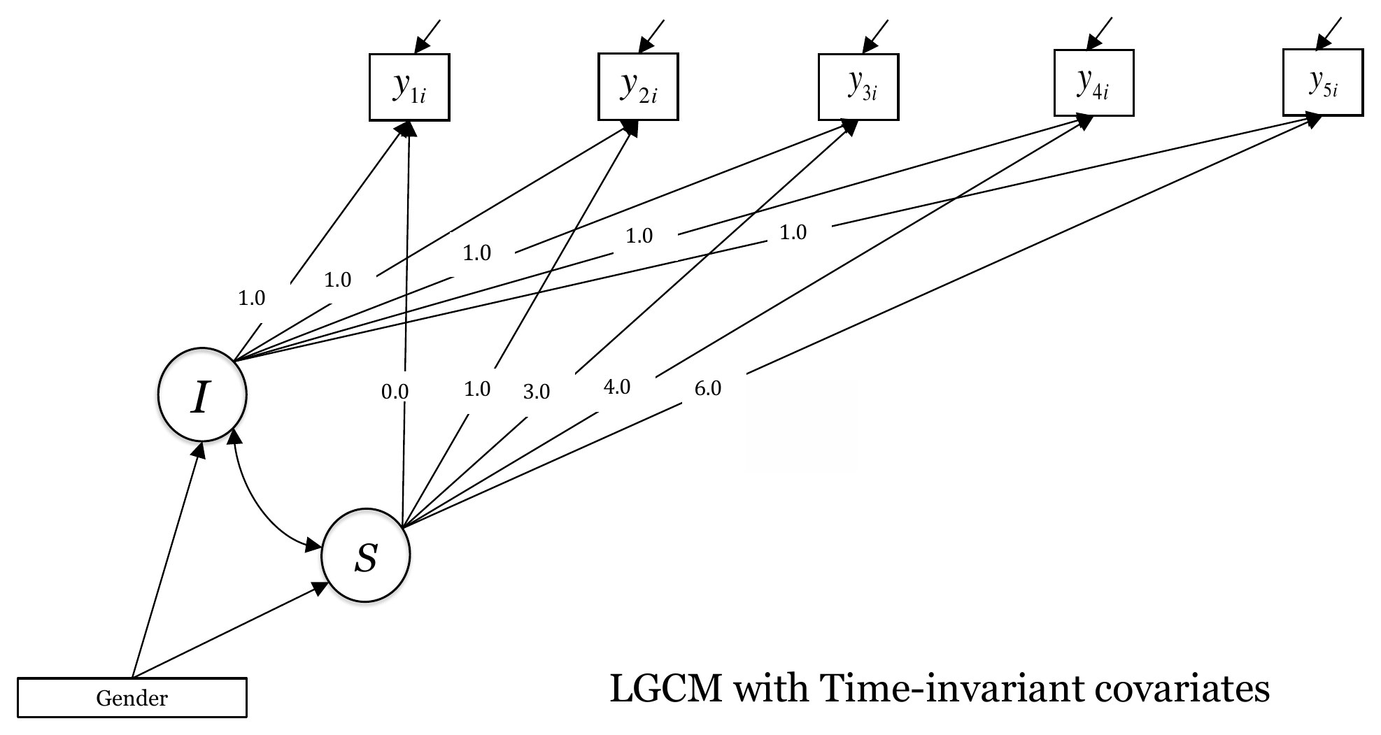
The dataset has 442 rows. The variable female is coded 0 for 222 rows and 1 for 193 rows, and it is missing for 27 rows. It is measured once, so every row carries a single value that applies to all five waves. The workshop slide shows the covariate in a box labeled Gender with one arrow to the intercept factor and one arrow to the slope factor (Figure 5.1). In this chapter we use the variable name female and its coding, and we describe differences only through the estimated coefficients.
The workshop script calls growth() with its default settings, so only rows with complete data on lone1 to lone5 and on female are used (see Chapter 1 for listwise deletion). Of the 442 rows, 121 lack at least one of the five loneliness scores, and 1 further row has all five scores but a missing female. The model is therefore estimated on 320 rows (178 coded 0 and 142 coded 1). The unconditional linear model of Chapter 2 used 321 rows, and this one row is the only difference in sample size between the two models.
5.4 The formal model
The measurement part is the same as in the linear growth model. The score of participant \(i\) at wave \(t\) is
\[ y_{ti} = \eta_{0i} + \lambda_t \, \eta_{1i} + \varepsilon_{ti}, \qquad \lambda_t = 0, 1, 3, 4, 6, \]
where \(\eta_{0i}\) is the intercept factor, \(\eta_{1i}\) is the slope factor, and the time scores \(\lambda_t\) follow the spacing of the waves. The structural part is new:
\[ \eta_{0i} = \alpha_0 + \gamma_0 \, \text{female}_i + \zeta_{0i}, \]
\[ \eta_{1i} = \alpha_1 + \gamma_1 \, \text{female}_i + \zeta_{1i}. \]
Here \(\alpha_0\) and \(\alpha_1\) are the conditional means of the growth factors, which are the expected intercept and slope for female = 0. The coefficients \(\gamma_0\) and \(\gamma_1\) are the differences in the expected intercept and slope between female = 1 and female = 0, because the covariate takes only the values 0 and 1. The terms \(\zeta_{0i}\) and \(\zeta_{1i}\) are the parts of the growth factors that female does not explain. Their variances are \(\psi_{00}\) and \(\psi_{11}\), and their covariance is \(\psi_{01}\). The residual variances of the five observed scores are freely estimated, as in the linear growth model.
The total variance of the intercept factor is the explained part plus the residual part,
\[ \mathrm{Var}(\eta_{0i}) = \gamma_0^2 \, \mathrm{Var}(\text{female}) + \psi_{00}, \]
and the same holds for the slope factor. The share of the total variance that is explained by female is therefore small whenever \(\gamma\) is small relative to the spread of the growth factor.
5.5 R implementation
The workshop syntax adds two regression lines to the linear growth model. In lavaan, ~ means “regressed on”. Because i and s are already defined as latent variables with =~, the two new lines are regressions of the growth factors on female. The covariate gets no loading and is not an indicator of the growth process.
Code
timeinvar <- ' i =~ 1*lone1 + 1*lone2 + 1*lone3 + 1*lone4 + 1*lone5
               s =~ 0*lone1 + 1*lone2 + 3*lone3 + 4*lone4 + 6*lone5

# Time invariant covariates
i ~ female
s ~ female'
fit_timeinvar <- growth(timeinvar, data = data)
summary(fit_timeinvar, fit.measures = TRUE)
lavaan 0.6.17 ended normally after 55 iterations
Estimator ML
Optimization method NLMINB
Number of model parameters 12
Used Total
Number of observations 320 442
Model Test User Model:
Test statistic 86.716
Degrees of freedom 13
P-value (Chi-square) 0.000
Model Test Baseline Model:
Test statistic 475.777
Degrees of freedom 15
P-value 0.000
User Model versus Baseline Model:
Comparative Fit Index (CFI) 0.840
Tucker-Lewis Index (TLI) 0.815
Loglikelihood and Information Criteria:
Loglikelihood user model (H0) -741.159
Loglikelihood unrestricted model (H1) -697.801
Akaike (AIC) 1506.319
Bayesian (BIC) 1551.538
Sample-size adjusted Bayesian (SABIC) 1513.476
Root Mean Square Error of Approximation:
RMSEA 0.133
90 Percent confidence interval - lower 0.107
90 Percent confidence interval - upper 0.160
P-value H_0: RMSEA <= 0.050 0.000
P-value H_0: RMSEA >= 0.080 1.000
Standardized Root Mean Square Residual:
SRMR 0.090
Parameter Estimates:
Standard errors Standard
Information Expected
Information saturated (h1) model Structured
Latent Variables:
Estimate Std.Err z-value P(>|z|)
i =~
lone1 1.000
lone2 1.000
lone3 1.000
lone4 1.000
lone5 1.000
s =~
lone1 0.000
lone2 1.000
lone3 3.000
lone4 4.000
lone5 6.000
Regressions:
Estimate Std.Err z-value P(>|z|)
i ~
female -0.132 0.047 -2.804 0.005
s ~
female 0.007 0.009 0.784 0.433
Covariances:
Estimate Std.Err z-value P(>|z|)
.i ~~
.s -0.015 0.002 -6.079 0.000
Intercepts:
Estimate Std.Err z-value P(>|z|)
.i 1.526 0.031 48.551 0.000
.s -0.029 0.006 -4.999 0.000
Variances:
Estimate Std.Err z-value P(>|z|)
.lone1 0.062 0.010 6.025 0.000
.lone2 0.112 0.011 10.064 0.000
.lone3 0.171 0.015 11.628 0.000
.lone4 0.107 0.010 10.953 0.000
.lone5 0.051 0.010 5.322 0.000
.i 0.134 0.015 9.164 0.000
.s 0.003 0.001 5.522 0.0005.6 Understanding the output
5.6.1 Fit
The output header shows that the model has 12 free parameters and uses 320 of 442 rows. Lavaan ended normally and gave no warning. The fit statistics are
- \(\chi^2\)(13) = 86.716, \(p\) < .001,
- CFI = 0.840 and TLI = 0.815,
- RMSEA = 0.133, 90% CI [0.107, 0.160],
- SRMR = 0.090.
Remember that only models with acceptable fit should be compared substantively. By the combination rules that are commonly attributed to Hu & Bentler (1999) (CFI near .95, RMSEA near .06, SRMR near .08), this model does not fit well, and the upper limit of the RMSEA interval is far above any usual threshold. Such cut-offs are guidelines and not fixed laws, but the distance here is large. The unconditional linear model of Chapter 2 had a CFI of 0.852, an RMSEA of 0.143 and an SRMR of 0.097. The two models fit about equally poorly, with a slightly lower CFI and a slightly lower RMSEA and SRMR for the covariate model. A covariate on the growth factors does not change the shape of change that the two factors can describe, so the misfit of the straight-line form is likely carried over into this model.
The degrees of freedom are 13 here and 10 in the linear model. The covariate adds five observed statistics (the associations between female and the five loneliness scores) and uses only two new parameters to reproduce them, so three degrees of freedom are gained. Because the two models differ in the variables that they contain, their chi-square values are not compared with a likelihood ratio test, and the fit indices above are only listed side by side.
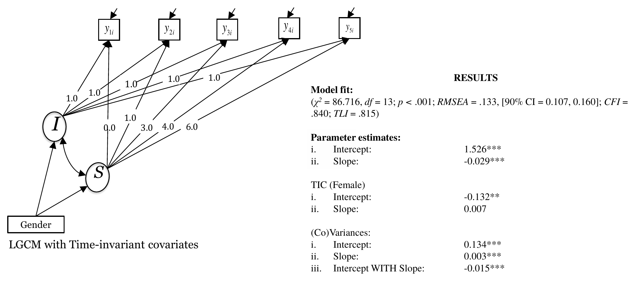
The slide with the results of the workshop is shown in Figure 5.2. It reports estimates that were computed in Mplus. The values on the slide agree with the lavaan output to three decimals, and the numbers used in this chapter are those of the R output.
The loneliness scores are skewed. Across the five waves the skewness ranges from 1.52 to 3.05 and the kurtosis from 2.27 to 12.75. The consequences for the chi-square statistic and the standard errors are described in Chapter 1. The poor fit may be partly due to this, and the standard errors below should be read as approximate.
5.6.2 The regression coefficients
The regressions are the new part of the output. Each row gives the expected difference in a growth factor for a one unit difference in female, which is the difference between the group coded 1 and the group coded 0.
female (listwise, N = 320).
| Path | Estimate | SE | \(z\) | \(p\) |
|---|---|---|---|---|
i ~ female |
-0.132 | 0.047 | -2.804 | 0.005 |
s ~ female |
0.007 | 0.009 | 0.784 | 0.433 |
5.6.3 Intercepts, variances and covariance
The intercepts of the growth factors are 1.526 for i and -0.029 for s. These are the conditional means for the participants coded 0. The variance of the residual of i is 0.134 and that of s is 0.003, and both are clearly different from zero. The covariance between the two residuals is -0.015. The variances of the residuals of the five loneliness scores are between 0.051 and 0.171.
To see what changed in the growth factors, we can place the conditional values next to the unconditional ones. The code below is an addition that was not part of the workshop. It fits the unconditional linear growth model to the same rows that the covariate model used, so that the two columns of the table come from identical data.
Code
# Addition (not part of the workshop): the linear growth model without the
# covariate, fitted to the same rows as the covariate model.
linear <- ' i =~ 1*lone1 + 1*lone2 + 1*lone3 + 1*lone4 + 1*lone5
            s =~ 0*lone1 + 1*lone2 + 3*lone3 + 4*lone4 + 6*lone5'
dat_used <- data[ok_model, ]
fit_linear_same <- growth(linear, data = dat_used)
pe_l <- parameterEstimates(fit_linear_same)
gl <- function(l, o, r) pe_l$est[pe_l$lhs == l & pe_l$op == o & pe_l$rhs == r]

cmp <- data.frame(
  Parameter = c("Mean of the intercept factor", "Mean of the slope factor",
                "Variance of the intercept factor", "Variance of the slope factor",
                "Covariance of the factors"),
  `Without covariate` = c(gl("i", "~1", ""), gl("s", "~1", ""),
                          gl("i", "~~", "i"), gl("s", "~~", "s"), gl("i", "~~", "s")),
  `With female` = c(a0, a1, psi0, psi1, psi01),
  check.names = FALSE)
cmp[, 2:3] <- lapply(cmp[, 2:3], round, 3)
knitr::kable(cmp, caption = "Growth factor parameters without and with the covariate (same rows). In the right column the means refer to female coded 0, and the variances and the covariance are residual values.")| Parameter | Without covariate | With female |
|---|---|---|
| Mean of the intercept factor | 1.467 | 1.526 |
| Mean of the slope factor | -0.025 | -0.029 |
| Variance of the intercept factor | 0.139 | 0.134 |
| Variance of the slope factor | 0.003 | 0.003 |
| Covariance of the factors | -0.015 | -0.015 |
The mean of the intercept factor goes from 1.467 to 1.526. This is not a contradiction. The unconditional mean is an average over both groups, and the conditional mean is the value for the group coded 0. We can recover the first from the second. The share of rows coded 1 among the rows used is 0.444, so the average of the two groups is \(1.526 + (-0.132)(0.444) = 1.467\). The variance of the intercept factor goes down from 0.139 to 0.134, and the proportion of the intercept variance that is explained by female is 0.031. For the slope factor the proportion is 0.004. Both proportions are small, and the second one is close to zero.
Coding and centering the covariate
The meaning of the intercept depends on the coding of female. With the 0 and 1 coding of the workshop, the intercept refers to the group coded 0. If the covariate is centered at its mean before it is used, the intercept refers to an average participant and equals the unconditional mean, while the regression coefficients stay the same. Centering is not part of the workshop syntax, so we only mention it here. Choose the coding that makes the intercept easiest to report, and say in the text which one was used.
5.7 Interpretation
The coefficient from female to i is -0.132 (SE = 0.047, \(z\) = -2.80, \(p\) = .005). The expected intercept is therefore about 0.13 units lower for the participants coded 1 than for the participants coded 0. The 95% confidence interval runs from -0.225 to -0.040, so the data are consistent with a difference that is anywhere from very small to about 0.22 units. The coefficient from female to s is 0.007 (SE = 0.009, \(p\) = .433). Its confidence interval, from -0.010 to 0.023, includes zero.
The slope difference is small in absolute terms. Over the six years that separate the first and the last wave, a difference of 0.007 per year adds up to about 0.04 units, compared with an intercept difference of 0.13. Table 5.2 and Figure 5.3 show what the estimates mean for the two groups. The expected trajectory of the group coded 0 starts at 1.526 and changes by -0.029 per year. The group coded 1 starts at 1.394 and changes by -0.022 per year. In both groups the expected score goes down over time, and the two lines are close to parallel, with the group coded 1 below the group coded 0 at every wave.
Code
imp <- data.frame(
  Group = c("female = 0", "female = 1"),
  Rows  = c(n_used_f0, n_used_f1),
  Intercept = c(a0, a0 + g0),
  Slope = c(a1, a1 + g1),
  `Expected, wave 1` = c(a0, a0 + g0),
  `Expected, wave 5` = c(a0 + 6 * a1, (a0 + g0) + 6 * (a1 + g1)),
  check.names = FALSE)
imp[, 3:6] <- lapply(imp[, 3:6], round, 3)
knitr::kable(imp)| Group | Rows | Intercept | Slope | Expected, wave 1 | Expected, wave 5 |
|---|---|---|---|---|---|
| female = 0 | 178 | 1.526 | -0.029 | 1.526 | 1.355 |
| female = 1 | 142 | 1.394 | -0.022 | 1.394 | 1.263 |
Code
tt <- 0:6
lines_df <- data.frame(
  time = rep(tt, 2),
  female = rep(c("0", "1"), each = length(tt)),
  mean = c(a0 + a1 * tt, (a0 + g0) + (a1 + g1) * tt))
obs_df <- dat_used |>
  pivot_longer(all_of(lone_vars), names_to = "wave", values_to = "lone") |>
  mutate(time = c(0, 1, 3, 4, 6)[as.integer(sub("lone", "", wave))],
         female = as.character(female)) |>
  group_by(female, time) |>
  summarise(mean = mean(lone), .groups = "drop")
ggplot(lines_df, aes(time, mean, color = female, linetype = female)) +
  geom_line(linewidth = 0.9) +
  geom_point(data = obs_df, size = 2.4) +
  scale_color_manual(values = c("0" = "black", "1" = "#B03A00")) +
  scale_linetype_manual(values = c("0" = "solid", "1" = "dashed")) +
  scale_x_continuous(breaks = c(0, 1, 3, 4, 6)) +
  labs(x = "Time (years since the first wave)", y = "Loneliness",
       color = "female", linetype = "female")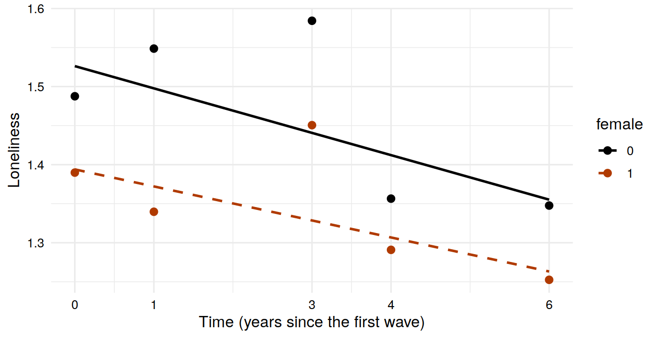
The observed means in Figure 5.3 do not follow the straight lines closely. In both groups the mean at the third wave lies above the line and the mean at the fourth wave lies below it, which is in line with the poor fit of the linear form. These findings should be read with this in mind. The regression coefficients are estimated under a linear model that does not describe the means and covariances of the data well. The sign and the rough size of the intercept difference are likely to be informative, but the exact value and the standard error depend on the model being adequate. The data suggest a lower starting level for the group coded 1 and do not provide evidence for a difference in the rate of change. They do not show that no such difference exists. The interval for the slope difference is wide enough to include small positive and small negative values.
The residual covariance between the factors is negative (-0.015). With the residual variances above, this corresponds to a correlation of about -0.72 between the parts of i and s that female does not explain. Participants with a higher starting level, given their value on female, tend to have a lower rate of change. This is the same pattern as in the linear growth model without the covariate.
5.8 Sensitivity to the missing data handling
This analysis is an addition to the workshop. The model above rests on listwise deletion, so 122 of the 442 rows are not used. We refit the model with full information maximum likelihood (FIML), which uses every row that has at least one observed value on the variables in the model. FIML was found to perform better than listwise deletion in the conditions examined by Enders & Bandalos (2001), and Enders (2010) gives an overview. The assumptions behind FIML and the missing data in this dataset are described in Chapter 1. The comparison here shows how much the answer depends on the handling of the missing values.
By default, lavaan treats female as a fixed predictor and deletes the rows in which it is missing, which would leave 415 rows. With fixed.x = FALSE, female is treated as a variable with a distribution, and the rows with a missing female are kept. The first fit below uses the workshop syntax and only changes the options. The second fit adds one line, female ~ 1, which frees the mean of female.
Code
# Addition (not part of the workshop): FIML sensitivity analysis.
# (1) workshop syntax, FIML, covariate treated as a random variable
fit_fiml <- growth(timeinvar, data = data, missing = "fiml", fixed.x = FALSE)

# (2) the same model with the mean of female estimated freely
timeinvar_mean <- paste(timeinvar, "\nfemale ~ 1")
fit_fiml_mean <- growth(timeinvar_mean, data = data, missing = "fiml", fixed.x = FALSE)
Lavaan prints a warning for the first fit. It says that the intercept of female is set to zero. In a growth model, lavaan sets the intercepts of the observed variables to zero, and this includes an observed covariate that has been added to the model as a random variable. The mean of female is 0.465 in the data, so the first FIML fit forces a mean of zero on a variable that does not have one. The warning about empty cases refers to rows that have no observed value on any variable in the model, and lavaan ignores them.
| Parameter | Listwise | FIML, mean of female fixed at 0 | FIML, mean of female free |
|---|---|---|---|
| i ~ female | -0.132 | -0.177 | -0.160 |
| s ~ female | 0.007 | 0.009 | 0.010 |
| Intercept of i (female = 0) | 1.526 | 1.569 | 1.564 |
| Intercept of s (female = 0) | -0.029 | -0.031 | -0.031 |
| Residual variance of i | 0.134 | 0.157 | 0.159 |
| Residual variance of s | 0.003 | 0.004 | 0.004 |
Rows used: 320 (listwise) and 439 (both FIML fits).
The point estimates are similar in the three versions. The coefficient from female to i is negative in all three versions (from -0.160 to -0.177 under FIML, against -0.132 listwise). The coefficient from female to s is small and positive in all three, between 0.007 and 0.010, and its standard error is of about the same size as the estimate in every version. The estimated intercept difference is somewhat larger in magnitude under FIML, although the gap between the versions is about one standard error of the listwise estimate or less. The conditional means of the growth factors change little. The residual variances are larger under FIML, 0.159 against 0.134 for the intercept factor. This may point to differences between the rows that were kept and the rows that were dropped, but these data cannot tell us why.
The FIML fit indices are not comparable with the listwise ones
The first FIML fit has a CFI of 0.450 and an RMSEA of 0.227 (chi-square 330.204 with 14 degrees of freedom), against a CFI of 0.840 and an RMSEA of 0.133 for the listwise model. This large difference does not mean that FIML made the model worse. With fixed.x = FALSE, the covariate is part of the model, so the fit statistics also test the mean and variance of female, and here the mean is forced to zero. When the mean is freed (second fit), the CFI is 0.891, the RMSEA is 0.105 and the SRMR is 0.074. This is closer to the listwise result, although the sample and the saturated model differ, so the indices are still not strictly comparable. Compare the point estimates across the handling methods, and judge the fit of the model from one version at a time.
5.9 What changed compared with the previous model
Compared with the unconditional linear model of Chapter 2, the measurement part is the same, and two regression paths have been added. The fit is similar, as discussed above, and the number of parameters goes from 10 to 12. The meaning of the growth factor means and variances has changed, as explained in the note earlier in the chapter.
Compared with the time-varying covariate model of Chapter 4, the covariate now explains differences between participants in the whole trajectory, and not differences between a score and the trajectory at one wave. A time-varying covariate speaks about what goes along with loneliness at the same wave. A time-invariant covariate speaks about who starts higher or changes faster. The two kinds of covariates are used together in Chapter 6.
The model differs from the multigroup approach of Chapter 8. Here, there is one growth model for all rows, and the only thing that is allowed to differ by female is the mean of each growth factor. The variances of the growth factors, their covariance and the residual variances of the five scores are held equal for the two groups. In the multigroup models of Chapter 8, these parameters can be freed one set at a time and tested.
The closest multigroup analogue of this chapter is model M2 of Chapter 8, in which the growth factor means are free and the variances and the covariance are held equal across groups. In M2 the intercept means are 1.550 for the group coded 0 and 1.401 for the group coded 1, and the slope means are -0.031 and -0.020. The differences between the groups, -0.149 for the intercept and 0.011 for the slope, have the same signs and a similar size as the coefficients of this chapter. The two sets of numbers are not strictly comparable. The multigroup models hold the residual variance of the loneliness scores equal across the five waves, which the covariate model does not, and they fit poorly.
The covariate approach uses fewer parameters than the multigroup approach, and a covariate does not have to be categorical.
5.10 What this model answers and what it cannot tell
The model answers whether a variable that is measured once is associated with the initial level of the growth process, with the rate of change, or with both. In this dataset, it suggests an association with the initial level and does not show one with the rate of change.
It cannot tell why the groups differ. A covariate such as female is a marker, and the regression says nothing about the reasons behind a difference. The model also does not say whether the groups differ in how much their members vary around the group trajectory, since the residual variances are held equal. Finally, the model describes a straight-line trajectory, which the fit indices do not support well, so the estimates are conditional on a shape that is questionable. They also depend on the 320 rows that were used.
5.11 Researcher’s perspective
A model with a time-invariant covariate needs one regression per growth factor and gives a direct answer about the initial level and the rate of change.
The coding of the covariate matters, since the intercept refers to the reference group and the interpretation of the growth factor means depends on it. Missing values need a decision as well. A covariate with missing values removes rows under listwise deletion, so report the number of rows used and the number of rows lost. In this dataset the loss caused by female is one row, and the loss caused by the loneliness scores is much larger. A FIML check, as in the sensitivity section, shows how much the conclusions depend on this choice. When you add a covariate to a FIML analysis in lavaan, remember that the mean of the covariate may have to be freed, and that fit indices from the two options cannot be compared.
The fit of this model is not good, so it may be better to improve the description of the shape of change first (Chapter 2 and the piecewise models of Chapter 3) and then add covariates. In the workshop, the covariate model is built on the linear form. Report both coefficients with their standard errors and not only the significant one, and describe the result in terms of the group coded 0 and the group coded 1.