The quadratic model of Chapter 2 lets the rate of change itself change, but it does so in one smooth curve over the whole observation period. A single polynomial cannot let the rate of change switch at a chosen time point. The piecewise growth model, also called the bilinear spline or multiphase growth model, can. It describes the trajectory with two linear pieces that are joined at one point, the knot, and it gives each piece its own slope factor (Flora, 2008).
The research question of this chapter is therefore the following. Is the average rate of change different before and after the knot, and do participants differ from each other in the rate of change in each of the two phases? The knot is chosen by the researcher, and so is the time point at which the intercept factor is defined. The chapter also shows how these two choices change what the parameters mean.
3.2 The idea in plain language
In the linear model we draw one straight line for each participant. In the piecewise model we draw two connected line segments. The first segment describes the change from the first wave up to the knot. The second segment describes the change from the knot up to the last wave. Because the segments are joined at the knot, the trajectory is continuous. It has a bend, but no jump.
Each segment has its own slope factor, and each participant can have a different slope in each phase. The two slopes are not forced to be related. A participant can change little in the early phase and more in the late phase, or the other way around. The model therefore has three growth factors: one intercept factor and two slope factors. We call them the early-phase slope and the late-phase slope.
The knot is a point that the researcher chooses. In practice, such a point may come from the design of a study (for example the time of a planned event or a change in conditions), from theory, or from the look of the plot of the wave means. In the workshop the knot was placed at the third wave, which is the year 2018, and we keep that choice here. The knot is placed at 2018 to show the model. It does not mean that something specific happens in 2018. Models in which the knot location is itself estimated also exist, but they are outside the workshop.
3.3 A concrete example with the dataset
We use the same data as in the previous chapters. Loneliness is measured at five waves, in 2015, 2016, 2018, 2019 and 2021. The spacing between waves is 1, 2, 1 and 2 years, and the time scores 0, 1, 3, 4 and 6 count the years since 2015. With the knot at the third wave (time score 3), the early phase covers the three years from 2015 to 2018 and the late phase covers the three years from 2018 to 2021. The two phases therefore have the same length in calendar time, which makes the two slopes easier to compare. Both are expressed as change per year.
The workshop script contains three versions of the model, which we call 4.1, 4.2 and 4.3. They all place the knot at 2018. They differ in the point in time at which the intercept is defined: 2015 in version 4.1, 2018 in version 4.2 and 2021 in version 4.3. The slides for these versions are shown later in the chapter, together with the output.
3.4 The formal model
For participant \(i\) at wave \(t\), the observed score is written as
Here \(\eta_{0i}\) is the intercept factor, \(\eta_{1i}\) and \(\eta_{2i}\) are the two slope factors, and the time scores \(\lambda_{1t}\) and \(\lambda_{2t}\) are fixed by the researcher. The growth factors have means \(\alpha_k\), and variances and covariances collected in a matrix \(\boldsymbol{\Psi}\). The residuals \(\varepsilon_{ti}\) have a freely estimated variance at each wave. The time scores of the three versions are given in Table 3.1.
Table 3.1: Time scores of the slope factors in the three versions. The loadings of the intercept factor are 1 at all waves in all versions.
Wave (year)
Time in years
4.1 s1
4.1 s2
4.2 s1
4.2 s2
4.3 s1
4.3 s2
1 (2015)
0
0
0
-3
0
-3
-3
2 (2016)
1
1
0
-2
0
-3
-2
3 (2018)
3
3
0
0
0
-3
0
4 (2019)
4
3
1
0
1
-2
0
5 (2021)
6
3
3
0
3
0
0
The columns of Table 3.1 can be written as simple functions of the time \(t\) in years, with the knot at \(t = 3\). In version 4.1, the early-phase slope has time scores \(\min(t, 3)\) and the late-phase slope has time scores \(\max(t - 3, 0)\). Notice what the flat parts of the columns mean. The early-phase slope stays at 3 after the knot. The factor then no longer adds anything to the predicted change after 2018, and what it contributed up to the knot is carried forward unchanged. The late-phase slope stays at 0 until the knot, so it has no effect before 2018 and starts to work afterwards.
In version 4.2 the time scores of the early-phase slope are \(\min(t, 3) - 3\), so they are zero at the knot. In version 4.3 both slopes are shifted so that they are zero at the last wave. There the early-phase slope has time scores \(\min(t, 3) - 3\) and the late-phase slope has time scores \(\max(t - 3, 0) - 3\). In the lavaan syntax of versions 4.1 and 4.2, s1 is the early-phase slope and s2 is the late-phase slope. In version 4.3 the labels are swapped, so that s1 is the late-phase slope and s2 is the early-phase slope. The diagram of version 4.3 in the workshop slides labels the early-phase slope as S1. In the text and in the tables we use the early-phase and late-phase names and follow the lavaan syntax when we refer to code.
Shifting the time scores by a constant changes the point at which the intercept factor is defined. Because \(\eta_{0} + \eta_{1}\lambda_{1} = (\eta_{0} + 3\eta_{1}) + \eta_{1}(\lambda_{1} - 3)\), the intercept factor of version 4.2 equals the intercept factor of version 4.1 plus three times the early-phase slope. The intercept factor of version 4.3 equals the one of version 4.1 plus three times the early-phase slope and three times the late-phase slope. The three versions are therefore the same model written with different growth factors. They imply the same means and the same covariance matrix of the five observed scores, and they have the same fit.
3.5 R implementation
The first step is to fit the three versions with the workshop syntax. The loadings are fixed by NUMBER*variable, as in the earlier chapters (Rosseel, 2012). The only change relative to the quadratic model is that there are now two slope factors.
3.5.1 Version 4.1: intercept in 2015, knot in 2018
lavaan 0.6.17 ended normally after 68 iterations

  Estimator                                         ML
  Optimization method                           NLMINB
  Number of model parameters                        14

                                                  Used       Total
  Number of observations                           321         442

Model Test User Model:

  Test statistic                                40.781
  Degrees of freedom                                 6
  P-value (Chi-square)                           0.000

Model Test Baseline Model:

  Test statistic                               451.170
  Degrees of freedom                                10
  P-value                                        0.000

User Model versus Baseline Model:

  Comparative Fit Index (CFI)                    0.921
  Tucker-Lewis Index (TLI)                       0.869

Loglikelihood and Information Criteria:

  Loglikelihood user model (H0)               -741.809
  Loglikelihood unrestricted model (H1)       -721.418

  Akaike (AIC)                                1511.618
  Bayesian (BIC)                              1564.418
  Sample-size adjusted Bayesian (SABIC)       1520.012

Root Mean Square Error of Approximation:

  RMSEA                                          0.134
  90 Percent confidence interval - lower         0.097
  90 Percent confidence interval - upper         0.175
  P-value H_0: RMSEA <= 0.050                    0.000
  P-value H_0: RMSEA >= 0.080                    0.991

Standardized Root Mean Square Residual:

  SRMR                                           0.074

Parameter Estimates:

  Standard errors                             Standard
  Information                                 Expected
  Information saturated (h1) model          Structured

Latent Variables:
                   Estimate  Std.Err  z-value  P(>|z|)
  i =~
    lone1             1.000
    lone2             1.000
    lone3             1.000
    lone4             1.000
    lone5             1.000
  s1 =~
    lone1            -3.000
    lone2            -3.000
    lone3            -3.000
    lone4            -2.000
    lone5             0.000
  s2 =~
    lone1            -3.000
    lone2            -2.000
    lone3             0.000
    lone4             0.000
    lone5             0.000

Covariances:
                   Estimate  Std.Err  z-value  P(>|z|)
  i ~~
    s1               -0.012    0.008   -1.377    0.168
    s2                0.011    0.003    3.342    0.001
  s1 ~~
    s2                0.000    0.002    0.083    0.934

Intercepts:
                   Estimate  Std.Err  z-value  P(>|z|)
    i                 1.288    0.019   68.489    0.000
    s1               -0.059    0.008   -7.002    0.000
    s2                0.007    0.008    0.807    0.420

Variances:
                   Estimate  Std.Err  z-value  P(>|z|)
   .lone1             0.046    0.012    3.772    0.000
   .lone2             0.114    0.011   10.134    0.000
   .lone3             0.130    0.016    8.057    0.000
   .lone4             0.106    0.011    9.719    0.000
   .lone5             0.082    0.022    3.665    0.000
    i                 0.036    0.022    1.637    0.102
    s1                0.002    0.004    0.571    0.568
    s2                0.008    0.002    3.404    0.001
3.6 Understanding the output
3.6.1 Sample size and warnings
Each of the three fits uses 321 of the 442 rows of the dataset, because growth() uses listwise deletion by default (see Chapter 1). The results are therefore about the participants with complete data on loneliness.
All three fits end normally, but lavaan prints a warning for each of them: the covariance matrix of the latent variables is not positive definite. Do not ignore this warning. A covariance matrix of the three growth factors that is not positive definite means that the estimates imply something impossible for the factors, for example a correlation larger than 1 in absolute value, or a negative variance. We can look at the implied matrix directly.
Code
# Addition to the workshop code: inspect the estimated covariance matrix of the growth factorslavInspect(fit_bilinear, "cov.lv")
        i     s1     s2
i   0.140
s1 -0.015  0.008
s2 -0.019  0.000  0.002
The smallest eigenvalue is slightly negative in all three versions, which is what the warning refers to. In version 4.1 the variance of the late-phase slope (s2) is 0.002, with a standard error of 0.004 and a p-value of .568. This variance is very close to zero, and it cannot be told apart from zero. At the same time, the covariance between the intercept factor and the late-phase slope is -0.019, which is large relative to the tiny variance of the slope. The implied correlation is -1.067, which is outside the range from -1 to 1. A correlation cannot be larger than 1 in absolute value, so the solution is inadmissible.
The same problem occurs in version 4.2, where the late-phase slope is the same factor, and in version 4.3, where the late-phase slope is labeled s1. The variance of the late-phase slope is the same in all three versions, since only the intercept factor is redefined.
A warning that does not go away
A non-positive definite covariance matrix of the latent variables means that at least one growth factor has too little variance to be estimated, and the covariances of that factor are then not trustworthy. The fit statistics and the means of the growth factors can still be reported, but the variance and covariance estimates involving the problematic factor should be reported with a clear note. Possible actions are to fix the variance of that factor to zero (with its covariances), to drop the factor, to simplify the model, or to use more data. None of these actions is free.
3.6.2 Fit
The fit statistics are identical across the three versions, and we take them from version 4.1. The chi-square test is \(\chi^2(6) = 40.781\), and it is the same for versions 4.2 and 4.3 (40.781 and 40.781). The p-value is below .001, so exact fit is rejected. The other indices are CFI \(= 0.921\), TLI \(= 0.869\), RMSEA \(= 0.134\) (90% CI [0.097, 0.175]) and SRMR \(= 0.074\).
By the usual cut-offs (Hu & Bentler, 1999), this is not a good fit. CFI is below .95, RMSEA is well above .08 and the whole confidence interval of RMSEA lies above .08. Only SRMR is close to the range that is usually considered acceptable. The model has 14 free parameters: three growth factor means, three variances, three covariances and five residual variances. With five waves there are 20 observed means, variances and covariances, so the model has \(20 - 14 = 6\) degrees of freedom. Remember that only models with acceptable fit should be interpreted substantively. We read the estimates below with this in mind, as a description of what the model implies for this dataset and not as firm conclusions.
The loneliness scores are skewed. The skewness of lone1 to lone5 ranges from 1.52 to 3.05, and the kurtosis goes up to 12.75. The chi-square test and the standard errors of maximum likelihood assume normally distributed data, and the chi-square statistic can be inflated with non-normal data (Curran et al., 1996). The size of the misfit may therefore be exaggerated, and the p-values below are approximate (see Chapter 1).
3.6.3 The same model in three coordinate systems
The estimates of the three versions differ, although the fit is identical. We collect the main ones in one table.
Table 3.2: Growth factor estimates of the three versions (listwise deletion). In version 4.3 the lavaan labels of the slopes are swapped, so the early-phase and late-phase slopes are listed by phase.
Parameter
4.1
4.2
4.3
Intercept mean
1.444
1.465
1.288
Early-phase slope mean
0.007
0.007
0.007
Late-phase slope mean
-0.059
-0.059
-0.059
Intercept variance
0.140
0.126
0.036
Early-phase slope variance
0.008
0.008
0.008
Late-phase slope variance
0.002
0.002
0.002
Intercept with early-phase slope
-0.015
0.010
0.011
Intercept with late-phase slope
-0.019
-0.018
-0.012
Early-phase with late-phase slope
0.000
0.000
0.000
The slope means and variances are the same in all three versions. The early-phase slope has a mean of 0.007 per year and the late-phase slope has a mean of -0.059 per year. What changes is everything that involves the intercept: its mean, its variance and its covariances with the slopes. The reason is that the intercept factor answers a different question in each version. We can verify this with the equations of the formal model. Starting from the estimates of version 4.1, we compute the intercept parameters of the other two versions and compare them with the estimates from the direct fits.
Code
est1 <-lavInspect(fit_bilinear, "est")alpha <-drop(est1$alpha) # means of i, s1, s2 in version 4.1psi <- est1$psi # (co)variances of i, s1, s2 in version 4.1# rows of W: new intercept, early-phase slope, late-phase slope, in terms of (i, s1, s2) of version 4.1W2 <-rbind(c(1, 3, 0), c(0, 1, 0), c(0, 0, 1)) # intercept in 2018W3 <-rbind(c(1, 3, 3), c(0, 1, 0), c(0, 0, 1)) # intercept in 2021d2 <- W2 %*% psi %*%t(W2); m2 <-drop(W2 %*% alpha)d3 <- W3 %*% psi %*%t(W3); m3 <-drop(W3 %*% alpha)reparam <-data.frame(Quantity =c("Intercept mean", "Intercept variance","Intercept with early-phase slope", "Intercept with late-phase slope"),`4.2 derived`=c(m2[1], d2[1, 1], d2[1, 2], d2[1, 3]),`4.2 estimated`=c(g(fit_bilinear_2, "i", "~1"), g(fit_bilinear_2, "i", "~~", "i"),g(fit_bilinear_2, "i", "~~", "s1"), g(fit_bilinear_2, "i", "~~", "s2")),`4.3 derived`=c(m3[1], d3[1, 1], d3[1, 2], d3[1, 3]),`4.3 estimated`=c(g(fit_bilinear_3, "i", "~1"), g(fit_bilinear_3, "i", "~~", "i"),g(fit_bilinear_3, "i", "~~", "s2"), g(fit_bilinear_3, "i", "~~", "s1")),check.names =FALSE)knitr::kable(reparam, digits =3)
Table 3.3: Intercept parameters of versions 4.2 and 4.3 derived from the estimates of version 4.1 and estimated directly. This check is an addition to the workshop code.
Quantity
4.2 derived
4.2 estimated
4.3 derived
4.3 estimated
Intercept mean
1.465
1.465
1.288
1.288
Intercept variance
0.126
0.126
0.036
0.036
Intercept with early-phase slope
0.010
0.010
0.011
0.011
Intercept with late-phase slope
-0.018
-0.018
-0.012
-0.012
The derived and the estimated values agree to the third decimal. The three versions are therefore reparameterizations of one model. Shifting the time scores by a constant leaves the model unchanged and moves the point to which the intercept factor refers.
3.7 Interpretation
3.7.1 Version 4.1: the starting level and two rates of change
In version 4.1 the intercept factor refers to the predicted average loneliness score in 2015. Its mean is 1.444 (standard error 0.024). The mean of the early-phase slope is 0.007 per year (standard error 0.008, p = .420). Over the three years of the early phase, this amounts to a predicted average change of about 0.021, which is small and is not distinguishable from zero. The mean of the late-phase slope is -0.059 per year (standard error 0.008, p < .001), which gives a predicted average decrease of about 0.176 over the three years from 2018 to 2021. For this dataset, then, the model describes an average trajectory that is roughly level until the knot and lower after it. This describes the average trajectory implied by the model and does not say why the scores change.
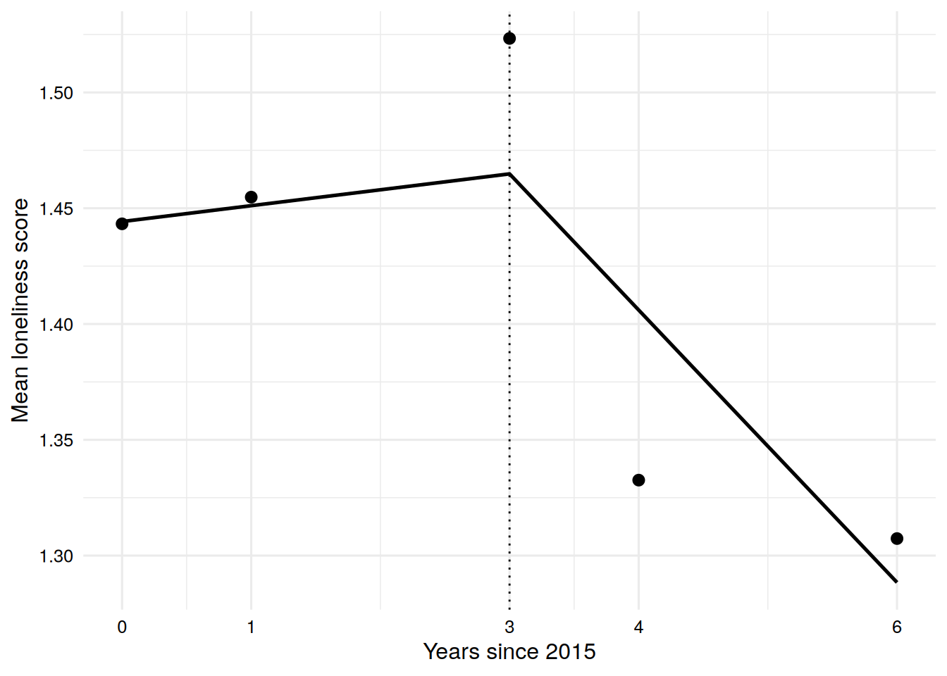
Figure 3.1 shows the observed means of the participants in the analysis next to the means implied by the model.
Code
means_df <-data.frame(years =c(0, 1, 3, 4, 6),observed =lavInspect(fit_bilinear, "sampstat")$mean,implied =fitted(fit_bilinear)$mean)ggplot(means_df, aes(x = years)) +geom_vline(xintercept =3, linetype ="dotted", color ="black") +geom_line(aes(y = implied), linewidth =0.9, color ="black") +geom_point(aes(y = observed), size =2.5, color ="black") +scale_x_continuous(breaks =c(0, 1, 3, 4, 6)) +labs(x ="Years since 2015", y ="Mean loneliness score")
Figure 3.1: Observed wave means (points) and the means implied by the bilinear model (line), plotted against years since 2015. The dotted vertical line marks the knot. Both come from the participants with complete data.
The implied line follows the observed means at the first, second and last wave closely. At the knot, however, the observed mean in 2018 (1.523) is higher than the implied mean (1.465), and in 2019 the observed mean (1.333) is lower than the implied mean (1.406). A trajectory that is joined at the knot cannot follow a peak in the observed means at the knot and a drop right after it. This is one place where the misfit of the model can be seen. It is also a reason not to read the early-phase slope as showing that nothing changes before 2018.
The covariance part of the output must be read with the warning in mind. The variance of the intercept factor is 0.140 (p < .001) and the variance of the early-phase slope is 0.008 (p = .001). Participants differ in the starting level and, to a small degree, in the rate of change before the knot. The variance of the late-phase slope is 0.002 and it is not distinguishable from zero. We cannot say from this model that participants differ in how quickly their scores change after the knot, and we also cannot say that they do not differ. The covariance of the intercept factor with the early-phase slope is -0.015 (implied correlation -0.438), so participants with a higher starting level tend to have a lower rate of change in the early phase. The covariance of the intercept factor with the late-phase slope is -0.019, but it is attached to a factor with almost no variance and an implied correlation beyond \(-1\). We do not interpret it. The covariance between the two slopes is 0.000 (p = .934).
Figure 3.2 shows the path diagram of version 4.1 and Figure 3.3 shows the slide with its results. The slide results come from Mplus. The estimates agree with the lavaan output in this chapter, with one exception. The slide gives 0.001 as the variance of the early-phase slope, while the lavaan output (and the slide of version 4.2) gives 0.008. The values of the R output are used in the text.
Figure 3.2: Version 4.1 of the bilinear spline model. Look at the loading columns next to the diagram: the early-phase slope increases to 3 at the knot and then stays at 3, and the late-phase slope is 0 until the knot and then increases. The intercept factor refers to the predicted average in 2015. Source: workshop slides (Anyan, 2023).
Figure 3.3: Results of version 4.1 as shown on the slide (estimated in Mplus). Compare the estimates with the lavaan output above. The numbers used in this chapter are those from the R output. Source: workshop slides (Anyan, 2023).
3.7.2 Version 4.2: the intercept at the knot
In version 4.2 the early-phase slope has time scores of \(-3, -2, 0, 0, 0\), so both slopes are zero in 2018. The intercept factor refers to the predicted average loneliness score in 2018, the year of the knot. Its mean is 1.465 (standard error 0.025). It is not a new finding. It equals the prediction of version 4.1 for 2018, namely \(1.444 + 3 \times 0.007 = 1.465\). The intercept variance is 0.126, a little smaller than in version 4.1.
The covariance of the intercept factor with the early-phase slope is now 0.010 (p = .045), whereas it was -0.015 in version 4.1. This is not a contradiction. In version 4.1 the covariance describes how the level in 2015 relates to the change from 2015 to 2018. In version 4.2 it describes how the level in 2018 relates to the same change, and a participant who is high in 2018 is partly high because of a positive change before 2018. The sign of an intercept-slope covariance depends on where the intercept is placed, and covariances from differently centered models cannot be compared directly (Biesanz et al., 2004). The problem with the late-phase slope remains.
Figure 3.4 and Figure 3.5 show the slides for this version. The numbers on the results slide agree with the lavaan output.
Figure 3.4: Version 4.2 of the spline model. The early-phase slope has negative time scores before the knot and zero afterwards, so that the intercept factor refers to the predicted average at the knot in 2018. Source: workshop slides (Anyan, 2023).
Figure 3.5: Results of version 4.2 as shown on the slide (estimated in Mplus). The chi-square, the slope means and the slope variances are the same as in version 4.1, and only the intercept parameters have changed. Source: workshop slides (Anyan, 2023).
3.7.3 Version 4.3: the intercept at the last wave
At the last wave, in 2021, both slopes are zero in version 4.3, so the intercept factor refers to the predicted average loneliness score at the end of the observation period. Its mean is 1.288 (standard error 0.019), which equals \(1.444 + 3 \times 0.007 + 3 \times (-0.059) = 1.288\) from version 4.1.
The two slopes carry swapped labels here. The factor s1 has the time scores \(-3, -3, -3, -2, 0\) and is the late-phase slope, with a mean of -0.059 and a variance of 0.002. The factor s2 has the time scores \(-3, -2, 0, 0, 0\) and is the early-phase slope, with a mean of 0.007 and a variance of 0.008. These are the same numbers as the ones of s2 and s1 in version 4.1. The diagram on the slide for this version (Figure 3.6) labels the slopes the other way round. The estimates on the results slide (Figure 3.7), for example the slope mean of -0.059 listed as Slope 1, follow the lavaan labeling.
The intercept variance in version 4.3 is 0.036 (standard error 0.022, p = .102), much smaller than in versions 4.1 and 4.2. It should not be read as a small difference between participants in 2021. It is the variance of the sum of the version 4.1 intercept factor, three times the early-phase slope and three times the late-phase slope. Its value comes from the variances and from the covariances of the three factors, and the covariance of the intercept factor with the late-phase slope is the one that is inadmissible in version 4.1. In version 4.3 the implied correlation between the intercept factor and the late-phase slope (s1) is -1.314, again beyond \(-1\). The small variance is therefore an artifact of the improper solution, and the FIML fit below gives a larger value. The covariance of the intercept factor with the early-phase slope is 0.011 (p = .001) and with the late-phase slope it is -0.012 (p = .168).
Figure 3.6: Version 4.3 of the spline model. Both slopes are zero at the last wave, so the intercept factor refers to the predicted average at the end of the observation period in 2021. In the diagram the early-phase slope, drawn with loadings -3, -2, 0, 0, 0, is labeled S1, whereas in the lavaan syntax these loadings belong to s2. Source: workshop slides (Anyan, 2023).
Figure 3.7: Results of version 4.3 as shown on the slide (estimated in Mplus). The slope with the mean of -0.059 is the late-phase slope, which is s1 in the lavaan syntax. The intercept variance of 0.036 agrees with the R output, and it is affected by the inadmissible solution described above. Source: workshop slides (Anyan, 2023).
Where to put the knot and where to put the intercept
These are two separate decisions. The knot is the point at which the rate of change is allowed to change. It should be based on the design or on theory, and it changes the model and its fit. The point at which the intercept factor is defined is a matter of interpretation, and it does not change the model or its fit. A useful habit is to choose the intercept factor so that the research question can be read from one parameter. If the question is about the level at the end of the study, version 4.3 is the natural choice. If the question is about the level at the knot, use version 4.2.
3.8 Comparing the bilinear model with the earlier models
The first three models are refitted here with the workshop syntax. The chi-square difference test and the information criteria below are an addition to the workshop code, which showed a comparison on a slide (Figure 3.8). The quadratic model gives the same warning about the latent covariance matrix as in Chapter 2.
Code
nogrowth <-' i =~ 1*lone1 + 1*lone2 + 1*lone3 + 1*lone4 + 1*lone5'fit_nogrowth <-growth(nogrowth, data = data)linear <-' i =~ 1*lone1 + 1*lone2 + 1*lone3 + 1*lone4 + 1*lone5 s =~ 0*lone1 + 1*lone2 + 3*lone3 + 4*lone4 + 6*lone5'fit_linear <-growth(linear, data = data)quadratic <-' i =~ 1*lone1 + 1*lone2 + 1*lone3 + 1*lone4 + 1*lone5 s =~ 0*lone1 + 1*lone2 + 3*lone3 + 4*lone4 + 6*lone5 q =~ 0*lone1 + 1*lone2 + 9*lone3 + 16*lone4 + 36*lone5'fit_quadratic <-growth(quadratic, data = data)# Addition to the workshop code: chi-square difference test of the linear against the bilinear modellrt <-anova(fit_bilinear, fit_linear)
The no growth, linear and quadratic models of Chapter 2 form a sequence of nested models. Each is a restricted version of the next, so the models can be compared with chi-square difference tests (Bentler & Bonett, 1980). The linear model is also nested in the bilinear model, because it is the bilinear model with the two slope factors set equal. This restriction removes 4 parameters. The chi-square difference is 34.46 on 4 degrees of freedom, and the reduced linear model is rejected, so the bilinear model fits better. The restriction puts a variance (that of the difference between the two slopes) on the boundary of its parameter space, so the p-value is only approximate (Self & Liang, 1987).
The bilinear and the quadratic model are not nested in each other. The bilinear model has 14 parameters and 6 degrees of freedom, exactly like the quadratic model, and neither is a restricted version of the other. The chi-square difference test is then not available, and the two models are compared with the information criteria AIC (Akaike, 1974) and BIC (Schwarz, 1978). Lower values are better, and the criteria penalize the number of parameters.
Table 3.4: Information criteria and fit of the models (listwise deletion). This table is an addition to the workshop code.
Model
Parameters
df
Chisq
AIC
BIC
CFI
RMSEA
No growth
7
13
186.433
1643.269
1669.669
0.607
0.204
Linear
10
10
75.244
1538.080
1575.795
0.852
0.143
Quadratic
14
6
46.671
1517.507
1570.308
0.908
0.145
Bilinear 4.1
14
6
40.781
1511.618
1564.418
0.921
0.134
Bilinear 4.2
14
6
40.781
1511.618
1564.418
0.921
0.134
Bilinear 4.3
14
6
40.781
1511.618
1564.418
0.921
0.134
Figure 3.8: Model comparison table from the workshop slides. The slide marks the bilinear spline model as non-nested with the earlier models and uses AIC and BIC. The linear model is nested in the bilinear model, as shown in the text. The AIC of the bilinear model on the slide (1511.809) and the chi-square of the no growth model (186.443) differ slightly from the lavaan values in Table 3.4. Source: workshop slides (Anyan, 2023).
The bilinear model has the lowest AIC (1511.618) and the lowest BIC (1564.418) of the models in the table. The quadratic model has an AIC of 1517.507 and a BIC of 1570.308. Since both models have the same number of parameters, the penalty terms cancel, and each criterion differs by 5.890, which is the difference between the two deviances. The comparison therefore favors the bilinear model, but the difference is modest. Both models fit poorly by the usual cut-offs and both give the same warning about the latent covariance matrix. The information criteria say which of the models describes the data better. They do not say that the best model fits well. The three versions have identical criteria in the table, as expected for the same model.
3.9 A check on the near-zero slope variance
The warning points to the variance of the late-phase slope. A natural reaction is to fix this variance to zero, which also fixes its covariances to zero, and to treat the late-phase slope as a fixed effect that is the same for every participant. The following code is an addition to the workshop code.
Code
# Addition to the workshop code (not part of the workshop script):# fix the variance of the late-phase slope, and its covariances, to zerobilinear_fixed <-paste(bilinear, "\n s2 ~~ 0*s2 + 0*i + 0*s1")fit_bilinear_fixed <-growth(bilinear_fixed, data = data)round(fitMeasures(fit_bilinear_fixed, c("chisq", "df", "cfi", "tli", "rmsea", "srmr", "aic", "bic")), 3)
The restriction removes 3 degrees of freedom. The chi-square increases from 40.781 to 77.117, CFI drops from 0.921 to 0.846 and RMSEA increases to 0.154. The model has no warning anymore, but its fit is worse than that of the unrestricted bilinear model and also worse than that of the linear model (chi-square 75.244 on 10 degrees of freedom, AIC 1538.080, against 77.117 on 9 degrees of freedom and AIC 1541.954). Part of the better fit of the unrestricted model may rest on the inadmissible covariance of the intercept factor with the late-phase slope, and these data cannot say more. The likelihood ratio test is not appropriate for a restriction that puts a variance at its boundary (Self & Liang, 1987), so we use the change in fit only descriptively.
Fixing the variance is therefore not a remedy here. The options are to report the original model with a clear description of the problem, to use a design with more waves in each phase so that each slope is based on more than three points, or to look for a different description of the change. Each phase here rests on only three waves, and the knot is shared by both phases. This limits how much information there is about the variance of each slope.
3.10 Sensitivity to the missing data handling
The results above use the participants with complete data on loneliness. As a check, which is an addition to the workshop, the three versions are refitted with full information maximum likelihood (FIML), which uses all available scores (see Chapter 1). lavaan ignores the rows without any loneliness score, so that 436 participants contribute.
# smallest eigenvalue of the latent covariance matrix under FIMLsapply(list(`4.1`= fit_bilinear_fiml, `4.2`= fit_bilinear_2_fiml, `4.3`= fit_bilinear_3_fiml),function(f) min(eigen(lavInspect(f, "cov.lv"))$values))
        4.1         4.2         4.3
0.001644986 0.001649265 0.004033187
The means of the growth factors change little. The intercept factor of version 4.1 has a mean of 1.464 under FIML (1.444 with listwise deletion), the early-phase slope has a mean of 0.008 (0.007) and the late-phase slope has a mean of -0.063 (-0.059). The variances are somewhat larger. The variance of the late-phase slope goes from 0.002 to 0.005 (p = .221), so it remains small and not distinguishable from zero. In version 4.3 the intercept variance is 0.073 under FIML (standard error 0.026), against 0.036 with listwise deletion. The smallest eigenvalue of the latent covariance matrix is positive in all three FIML fits, so the warning does not appear. The chi-square values of the two analyses are not compared, since they are based on different numbers of participants.
A second check changes the estimator. FIML with the robust maximum likelihood estimator MLR(Yuan & Bentler, 2000) gives the following fit for version 4.1.
Code
# Addition to the workshop code: FIML with a robust estimatorfit_bilinear_mlr <-growth(bilinear, data = data, missing ="fiml", estimator ="MLR")round(fitMeasures(fit_bilinear_mlr, c("chisq.scaled", "df.scaled", "cfi.robust", "rmsea.robust")), 3)
The scaled chi-square is 15.762, compared with 31.360 for the FIML fit with the standard chi-square on the same participants. The robust CFI is 0.966 and the robust RMSEA is 0.093. The smaller scaled statistic is what is expected with skewed scores (see Chapter 1).
3.11 What changed compared with the previous model
The quadratic model of Chapter 2 and the bilinear model have the same number of parameters and the same degrees of freedom. The difference lies in the shape of the average trajectory. The quadratic model describes one smooth curve and the bilinear model describes two straight pieces with a bend at the knot. The chi-square drops from 46.671 to 40.781, and the information criteria favor the bilinear model slightly. Compared with the linear model, the bilinear model allows the average rate of change to differ between the two phases and adds a second slope factor, with its variance and covariances. The bilinear model fits better than the linear model, but the data do not show whether this comes from the different means of the two phases, from the extra slope factor, or from the inadmissible solution. The extra slope factor is also the source of the warning, because it has to be estimated from three waves.
3.12 What this model answers and what it cannot tell
The model answers whether the average rate of change differs between the two phases and whether participants differ in the rate of change in each phase, given a knot that the researcher has chosen. For this dataset and the knot at the third wave, the average rate before the knot is small and the average rate after it is negative. Participants differ in the starting level and, slightly, in the early-phase rate, but the data do not settle whether they differ in the late-phase rate.
The model does not tell why the rate of change differs between the phases, and it does not tell that anything happens at the knot. The knot at the third wave was fixed in advance, and other knot positions were not compared. With only five waves, the choices for the knot are few. The fit is poor by the usual cut-offs, so the model does not describe the covariance structure of the five waves well. The non-positive definite covariance matrix means that the variance and covariance estimates involving the late-phase slope are not reliable. The three versions of the model cannot be told apart by fit, so the choice among them is a choice of interpretation and not a result.
3.13 Researcher’s perspective
The location of the knot should be motivated before the analysis, by the design or by theory, and it should be stated in the report as a choice. If several knot locations are tried, say so, since trying many and reporting the best one overstates the evidence.
Because the three versions have the same fit, choose the version in which the parameter of interest is in the intercept factor, and say where the intercept factor is located. When intercept-slope covariances are reported, state the point in time to which they refer, since the sign can change with the centering. If you compare your results with the literature, check how time was coded there.
A warning about the latent covariance matrix is part of the results and should be reported with the variance estimate that causes it, together with what was done about it. Here the near-zero variance of the late-phase slope prevents strong statements about individual differences in that phase. Fixing the variance to zero made the fit worse, and the FIML analysis removed the warning. Both facts belong in the write-up. Report that listwise deletion was used, give the number of participants analyzed, and give the FIML result as a check (Chapter 1).
The next chapter adds a second variable that is measured at every wave, a time-varying covariate (Chapter 4).
Akaike, H. (1974). A new look at the statistical model identification. IEEE Transactions on Automatic Control, 19(6), 716–723. https://doi.org/10.1109/TAC.1974.1100705
Anyan, F. (2023). Longitudinal data analysis using Mplus and R. Workshop slides.
Bentler, P. M., & Bonett, D. G. (1980). Significance tests and goodness of fit in the analysis of covariance structures. Psychological Bulletin, 88(3), 588–606. https://doi.org/10.1037/0033-2909.88.3.588
Biesanz, J. C., Deeb-Sossa, N., Papadakis, A. A., Bollen, K. A., & Curran, P. J. (2004). The role of coding time in estimating and interpreting growth curve models. Psychological Methods, 9(1), 30–52. https://doi.org/10.1037/1082-989X.9.1.30
Curran, P. J., West, S. G., & Finch, J. F. (1996). The robustness of test statistics to nonnormality and specification error in confirmatory factor analysis. Psychological Methods, 1(1), 16–29. https://doi.org/10.1037/1082-989X.1.1.16
Flora, D. B. (2008). Specifying piecewise latent trajectory models for longitudinal data. Structural Equation Modeling: A Multidisciplinary Journal, 15(3), 513–533. https://doi.org/10.1080/10705510802154349
Hu, L., & Bentler, P. M. (1999). Cutoff criteria for fit indexes in covariance structure analysis: Conventional criteria versus new alternatives. Structural Equation Modeling: A Multidisciplinary Journal, 6(1), 1–55. https://doi.org/10.1080/10705519909540118
Rosseel, Y. (2012). lavaan: An R package for structural equation modeling. Journal of Statistical Software, 48(2), 1–36. https://doi.org/10.18637/jss.v048.i02
Schwarz, G. (1978). Estimating the dimension of a model. The Annals of Statistics, 6(2), 461–464.
Self, S. G., & Liang, K.-Y. (1987). Asymptotic properties of maximum likelihood estimators and likelihood ratio tests under nonstandard conditions. Journal of the American Statistical Association, 82(398), 605–610. https://doi.org/10.1080/01621459.1987.10478472
Yuan, K.-H., & Bentler, P. M. (2000). Three likelihood-based methods for mean and covariance structure analysis with nonnormal missing data. Sociological Methodology, 30, 165–200.
Source Code
# Piecewise and spline growth models {#sec-piecewise}```{r}#| label: setup#| include: falselibrary(lavaan)library(dplyr)library(tidyr)library(ggplot2)library(psych)data <-read.csv("data/data.csv", fileEncoding ="UTF-8-BOM")theme_set(theme_minimal(base_size =12) +theme(plot.title =element_text(face ="bold", color ="black"),axis.title =element_text(color ="black"),axis.text =element_text(color ="black"),strip.text =element_text(color ="black"),legend.text =element_text(color ="black")))``````{r}#| label: helpers#| include: false# small helpers used only for inline numbers in the textf3 <-function(x) formatC(x, format ="f", digits =3)fp <-function(x) sub("^0", "", f3(x)) # p-values without the leading zero# estimate, standard error and p-value of one parameterg <-function(fit, lhs, op, rhs ="") { p <-parameterEstimates(fit) p[p$lhs == lhs & p$op == op & p$rhs == rhs, "est"]}gse <-function(fit, lhs, op, rhs ="") { p <-parameterEstimates(fit) p[p$lhs == lhs & p$op == op & p$rhs == rhs, "se"]}gp <-function(fit, lhs, op, rhs ="") { p <-parameterEstimates(fit) p[p$lhs == lhs & p$op == op & p$rhs == rhs, "pvalue"]}fmx <-function(fit, m, d =3) formatC(unname(fitMeasures(fit, m)), format ="f", digits = d)f2 <-function(x) formatC(x, format ="f", digits =2)d_lone <- psych::describe(data[, paste0("lone", 1:5)]) # skewness and kurtosis of the five scores```## Why this modelThe quadratic model of @sec-basic lets the rate of change itself change, but it does so in one smooth curve over the whole observation period. A single polynomial cannot let the rate of change switch at a chosen time point. The *piecewise growth model*, also called the *bilinear spline* or *multiphase* growth model, can. It describes the trajectory with two linear pieces that are joined at one point, the *knot*, and it gives each piece its own slope factor [@flora2008piecewise].The research question of this chapter is therefore the following. Is the average rate of change different before and after the knot, and do participants differ from each other in the rate of change in each of the two phases? The knot is chosen by the researcher, and so is the time point at which the intercept factor is defined. The chapter also shows how these two choices change what the parameters mean.## The idea in plain languageIn the linear model we draw one straight line for each participant. In the piecewise model we draw two connected line segments. The first segment describes the change from the first wave up to the knot. The second segment describes the change from the knot up to the last wave. Because the segments are joined at the knot, the trajectory is continuous. It has a bend, but no jump.Each segment has its own slope factor, and each participant can have a different slope in each phase. The two slopes are not forced to be related. A participant can change little in the early phase and more in the late phase, or the other way around. The model therefore has three growth factors: one intercept factor and two slope factors. We call them the early-phase slope and the late-phase slope.The knot is a point that the researcher chooses. In practice, such a point may come from the design of a study (for example the time of a planned event or a change in conditions), from theory, or from the look of the plot of the wave means. In the workshop the knot was placed at the third wave, which is the year 2018, and we keep that choice here. The knot is placed at 2018 to show the model. It does not mean that something specific happens in 2018. Models in which the knot location is itself estimated also exist, but they are outside the workshop.## A concrete example with the datasetWe use the same data as in the previous chapters. Loneliness is measured at five waves, in 2015, 2016, 2018, 2019 and 2021. The spacing between waves is 1, 2, 1 and 2 years, and the time scores 0, 1, 3, 4 and 6 count the years since 2015. With the knot at the third wave (time score 3), the early phase covers the three years from 2015 to 2018 and the late phase covers the three years from 2018 to 2021. The two phases therefore have the same length in calendar time, which makes the two slopes easier to compare. Both are expressed as change per year.The workshop script contains three versions of the model, which we call 4.1, 4.2 and 4.3. They all place the knot at 2018. They differ in the point in time at which the intercept is defined: 2015 in version 4.1, 2018 in version 4.2 and 2021 in version 4.3. The slides for these versions are shown later in the chapter, together with the output.## The formal modelFor participant $i$ at wave $t$, the observed score is written as$$y_{ti} = \eta_{0i} + \eta_{1i}\,\lambda_{1t} + \eta_{2i}\,\lambda_{2t} + \varepsilon_{ti}.$$Here $\eta_{0i}$ is the intercept factor, $\eta_{1i}$ and $\eta_{2i}$ are the two slope factors, and the time scores $\lambda_{1t}$ and $\lambda_{2t}$ are fixed by the researcher. The growth factors have means $\alpha_k$, and variances and covariances collected in a matrix $\boldsymbol{\Psi}$. The residuals $\varepsilon_{ti}$ have a freely estimated variance at each wave. The time scores of the three versions are given in @tbl-timescores.| Wave (year) | Time in years | 4.1 s1 | 4.1 s2 | 4.2 s1 | 4.2 s2 | 4.3 s1 | 4.3 s2 ||---|---|---|---|---|---|---|---|| 1 (2015) | 0 | 0 | 0 | -3 | 0 | -3 | -3 || 2 (2016) | 1 | 1 | 0 | -2 | 0 | -3 | -2 || 3 (2018) | 3 | 3 | 0 | 0 | 0 | -3 | 0 || 4 (2019) | 4 | 3 | 1 | 0 | 1 | -2 | 0 || 5 (2021) | 6 | 3 | 3 | 0 | 3 | 0 | 0 |: Time scores of the slope factors in the three versions. The loadings of the intercept factor are 1 at all waves in all versions. {#tbl-timescores}The columns of @tbl-timescores can be written as simple functions of the time $t$ in years, with the knot at $t = 3$. In version 4.1, the early-phase slope has time scores $\min(t, 3)$ and the late-phase slope has time scores $\max(t - 3, 0)$. Notice what the flat parts of the columns mean. The early-phase slope stays at 3 after the knot. The factor then no longer adds anything to the predicted change after 2018, and what it contributed up to the knot is carried forward unchanged. The late-phase slope stays at 0 until the knot, so it has no effect before 2018 and starts to work afterwards.In version 4.2 the time scores of the early-phase slope are $\min(t, 3) - 3$, so they are zero at the knot. In version 4.3 both slopes are shifted so that they are zero at the last wave. There the early-phase slope has time scores $\min(t, 3) - 3$ and the late-phase slope has time scores $\max(t - 3, 0) - 3$. In the lavaan syntax of versions 4.1 and 4.2, `s1` is the early-phase slope and `s2` is the late-phase slope. In version 4.3 the labels are swapped, so that `s1` is the late-phase slope and `s2` is the early-phase slope. The diagram of version 4.3 in the workshop slides labels the early-phase slope as S1. In the text and in the tables we use the early-phase and late-phase names and follow the lavaan syntax when we refer to code.Shifting the time scores by a constant changes the point at which the intercept factor is defined. Because $\eta_{0} + \eta_{1}\lambda_{1} = (\eta_{0} + 3\eta_{1}) + \eta_{1}(\lambda_{1} - 3)$, the intercept factor of version 4.2 equals the intercept factor of version 4.1 plus three times the early-phase slope. The intercept factor of version 4.3 equals the one of version 4.1 plus three times the early-phase slope and three times the late-phase slope. The three versions are therefore the same model written with different growth factors. They imply the same means and the same covariance matrix of the five observed scores, and they have the same fit.## R implementationThe first step is to fit the three versions with the workshop syntax. The loadings are fixed by `NUMBER*variable`, as in the earlier chapters [@rosseel2012lavaan]. The only change relative to the quadratic model is that there are now two slope factors.### Version 4.1: intercept in 2015, knot in 2018```{r}#| label: bilinearbilinear <-' i =~ 1*lone1 + 1*lone2 + 1*lone3 + 1*lone4 + 1*lone5 s1 =~ 0*lone1 + 1*lone2 + 3*lone3 + 3*lone4 + 3*lone5 s2 =~ 0*lone1 + 0*lone2 + 0*lone3 + 1*lone4 + 3*lone5'fit_bilinear <-growth(bilinear, data = data)summary(fit_bilinear, fit.measures =TRUE)```### Version 4.2: intercept in 2018, knot in 2018```{r}#| label: bilinear-2bilinear_2 <-' i =~ 1*lone1 + 1*lone2 + 1*lone3 + 1*lone4 + 1*lone5 s1 =~ -3*lone1 + -2*lone2 + 0*lone3 + 0*lone4 + 0*lone5 s2 =~ 0*lone1 + 0*lone2 + 0*lone3 + 1*lone4 + 3*lone5'fit_bilinear_2 <-growth(bilinear_2, data = data)summary(fit_bilinear_2, fit.measures =TRUE)```### Version 4.3: intercept in 2021, knot in 2018```{r}#| label: bilinear-3bilinear_3 <-' i =~ 1*lone1 + 1*lone2 + 1*lone3 + 1*lone4 + 1*lone5 s1 =~ -3*lone1 + -3*lone2 + -3*lone3 + -2*lone4 + 0*lone5 s2 =~ -3*lone1 + -2*lone2 + 0*lone3 + 0*lone4 + 0*lone5'fit_bilinear_3 <-growth(bilinear_3, data = data)summary(fit_bilinear_3, fit.measures =TRUE)```## Understanding the output### Sample size and warningsEach of the three fits uses `r lavInspect(fit_bilinear, "nobs")` of the `r nrow(data)` rows of the dataset, because `growth()` uses listwise deletion by default (see @sec-prelims). The results are therefore about the participants with complete data on loneliness.All three fits end normally, but lavaan prints a warning for each of them: the covariance matrix of the latent variables is not positive definite. Do not ignore this warning. A covariance matrix of the three growth factors that is not positive definite means that the estimates imply something impossible for the factors, for example a correlation larger than 1 in absolute value, or a negative variance. We can look at the implied matrix directly.```{r}#| label: check-cov-lv# Addition to the workshop code: inspect the estimated covariance matrix of the growth factorslavInspect(fit_bilinear, "cov.lv")cor2 <-cov2cor(lavInspect(fit_bilinear, "cov.lv"))round(cor2, 3)chk <-sapply(list(`4.1`= fit_bilinear, `4.2`= fit_bilinear_2, `4.3`= fit_bilinear_3),function(f) { S <-lavInspect(f, "cov.lv") R <-cov2cor(S)c(smallest_eigenvalue =min(eigen(S)$values),smallest_variance =min(diag(S)),largest_abs_cor =max(abs(R[lower.tri(R)]))) })round(t(chk), 4)```The smallest eigenvalue is slightly negative in all three versions, which is what the warning refers to. In version 4.1 the variance of the late-phase slope (`s2`) is `r f3(g(fit_bilinear, "s2", "~~", "s2"))`, with a standard error of `r f3(gse(fit_bilinear, "s2", "~~", "s2"))` and a *p*-value of `r fp(gp(fit_bilinear, "s2", "~~", "s2"))`. This variance is very close to zero, and it cannot be told apart from zero. At the same time, the covariance between the intercept factor and the late-phase slope is `r f3(g(fit_bilinear, "i", "~~", "s2"))`, which is large relative to the tiny variance of the slope. The implied correlation is `r f3(cor2["i", "s2"])`, which is outside the range from -1 to 1. A correlation cannot be larger than 1 in absolute value, so the solution is inadmissible.The same problem occurs in version 4.2, where the late-phase slope is the same factor, and in version 4.3, where the late-phase slope is labeled `s1`. The variance of the late-phase slope is the same in all three versions, since only the intercept factor is redefined.::: {.callout-warning title="A warning that does not go away"}A non-positive definite covariance matrix of the latent variables means that at least one growth factor has too little variance to be estimated, and the covariances of that factor are then not trustworthy. The fit statistics and the means of the growth factors can still be reported, but the variance and covariance estimates involving the problematic factor should be reported with a clear note. Possible actions are to fix the variance of that factor to zero (with its covariances), to drop the factor, to simplify the model, or to use more data. None of these actions is free.:::### FitThe fit statistics are identical across the three versions, and we take them from version 4.1. The chi-square test is $\chi^2(`r fitMeasures(fit_bilinear, "df")`) = `r fmx(fit_bilinear, "chisq")`$, and it is the same for versions 4.2 and 4.3 (`r fmx(fit_bilinear_2, "chisq")` and `r fmx(fit_bilinear_3, "chisq")`). The *p*-value is below .001, so exact fit is rejected. The other indices are CFI $= `r fmx(fit_bilinear, "cfi")`$, TLI $= `r fmx(fit_bilinear, "tli")`$, RMSEA $= `r fmx(fit_bilinear, "rmsea")`$ (90% CI [`r fmx(fit_bilinear, "rmsea.ci.lower")`, `r fmx(fit_bilinear, "rmsea.ci.upper")`]) and SRMR $= `r fmx(fit_bilinear, "srmr")`$.By the usual cut-offs [@hu1999cutoff], this is not a good fit. CFI is below .95, RMSEA is well above .08 and the whole confidence interval of RMSEA lies above .08. Only SRMR is close to the range that is usually considered acceptable. The model has `r fitMeasures(fit_bilinear, "npar")` free parameters: three growth factor means, three variances, three covariances and five residual variances. With five waves there are `r 5 + choose(5, 2) + 5` observed means, variances and covariances, so the model has $`r 5 + choose(5, 2) + 5` - `r fitMeasures(fit_bilinear, "npar")` = `r fitMeasures(fit_bilinear, "df")`$ degrees of freedom. Remember that only models with acceptable fit should be interpreted substantively. We read the estimates below with this in mind, as a description of what the model implies for this dataset and not as firm conclusions.The loneliness scores are skewed. The skewness of `lone1` to `lone5` ranges from `r f2(min(d_lone$skew))` to `r f2(max(d_lone$skew))`, and the kurtosis goes up to `r f2(max(d_lone$kurtosis))`. The chi-square test and the standard errors of maximum likelihood assume normally distributed data, and the chi-square statistic can be inflated with non-normal data [@curran1996robustness]. The size of the misfit may therefore be exaggerated, and the *p*-values below are approximate (see @sec-prelims).### The same model in three coordinate systemsThe estimates of the three versions differ, although the fit is identical. We collect the main ones in one table.```{r}#| label: tbl-estimates#| tbl-cap: "Growth factor estimates of the three versions (listwise deletion). In version 4.3 the lavaan labels of the slopes are swapped, so the early-phase and late-phase slopes are listed by phase."est_tab <-data.frame(Parameter =c("Intercept mean", "Early-phase slope mean", "Late-phase slope mean","Intercept variance", "Early-phase slope variance", "Late-phase slope variance","Intercept with early-phase slope", "Intercept with late-phase slope","Early-phase with late-phase slope"),`4.1`=c(g(fit_bilinear, "i", "~1"), g(fit_bilinear, "s1", "~1"), g(fit_bilinear, "s2", "~1"),g(fit_bilinear, "i", "~~", "i"), g(fit_bilinear, "s1", "~~", "s1"), g(fit_bilinear, "s2", "~~", "s2"),g(fit_bilinear, "i", "~~", "s1"), g(fit_bilinear, "i", "~~", "s2"), g(fit_bilinear, "s1", "~~", "s2")),`4.2`=c(g(fit_bilinear_2, "i", "~1"), g(fit_bilinear_2, "s1", "~1"), g(fit_bilinear_2, "s2", "~1"),g(fit_bilinear_2, "i", "~~", "i"), g(fit_bilinear_2, "s1", "~~", "s1"), g(fit_bilinear_2, "s2", "~~", "s2"),g(fit_bilinear_2, "i", "~~", "s1"), g(fit_bilinear_2, "i", "~~", "s2"), g(fit_bilinear_2, "s1", "~~", "s2")),`4.3`=c(g(fit_bilinear_3, "i", "~1"), g(fit_bilinear_3, "s2", "~1"), g(fit_bilinear_3, "s1", "~1"),g(fit_bilinear_3, "i", "~~", "i"), g(fit_bilinear_3, "s2", "~~", "s2"), g(fit_bilinear_3, "s1", "~~", "s1"),g(fit_bilinear_3, "i", "~~", "s2"), g(fit_bilinear_3, "i", "~~", "s1"), g(fit_bilinear_3, "s1", "~~", "s2")),check.names =FALSE)knitr::kable(est_tab, digits =3)```The slope means and variances are the same in all three versions. The early-phase slope has a mean of `r f3(g(fit_bilinear, "s1", "~1"))` per year and the late-phase slope has a mean of `r f3(g(fit_bilinear, "s2", "~1"))` per year. What changes is everything that involves the intercept: its mean, its variance and its covariances with the slopes. The reason is that the intercept factor answers a different question in each version. We can verify this with the equations of the formal model. Starting from the estimates of version 4.1, we compute the intercept parameters of the other two versions and compare them with the estimates from the direct fits.```{r}#| label: tbl-reparam#| tbl-cap: "Intercept parameters of versions 4.2 and 4.3 derived from the estimates of version 4.1 and estimated directly. This check is an addition to the workshop code."est1 <-lavInspect(fit_bilinear, "est")alpha <-drop(est1$alpha) # means of i, s1, s2 in version 4.1psi <- est1$psi # (co)variances of i, s1, s2 in version 4.1# rows of W: new intercept, early-phase slope, late-phase slope, in terms of (i, s1, s2) of version 4.1W2 <-rbind(c(1, 3, 0), c(0, 1, 0), c(0, 0, 1)) # intercept in 2018W3 <-rbind(c(1, 3, 3), c(0, 1, 0), c(0, 0, 1)) # intercept in 2021d2 <- W2 %*% psi %*%t(W2); m2 <-drop(W2 %*% alpha)d3 <- W3 %*% psi %*%t(W3); m3 <-drop(W3 %*% alpha)reparam <-data.frame(Quantity =c("Intercept mean", "Intercept variance","Intercept with early-phase slope", "Intercept with late-phase slope"),`4.2 derived`=c(m2[1], d2[1, 1], d2[1, 2], d2[1, 3]),`4.2 estimated`=c(g(fit_bilinear_2, "i", "~1"), g(fit_bilinear_2, "i", "~~", "i"),g(fit_bilinear_2, "i", "~~", "s1"), g(fit_bilinear_2, "i", "~~", "s2")),`4.3 derived`=c(m3[1], d3[1, 1], d3[1, 2], d3[1, 3]),`4.3 estimated`=c(g(fit_bilinear_3, "i", "~1"), g(fit_bilinear_3, "i", "~~", "i"),g(fit_bilinear_3, "i", "~~", "s2"), g(fit_bilinear_3, "i", "~~", "s1")),check.names =FALSE)knitr::kable(reparam, digits =3)```The derived and the estimated values agree to the third decimal. The three versions are therefore reparameterizations of one model. Shifting the time scores by a constant leaves the model unchanged and moves the point to which the intercept factor refers.## Interpretation### Version 4.1: the starting level and two rates of changeIn version 4.1 the intercept factor refers to the predicted average loneliness score in 2015. Its mean is `r f3(g(fit_bilinear, "i", "~1"))` (standard error `r f3(gse(fit_bilinear, "i", "~1"))`). The mean of the early-phase slope is `r f3(g(fit_bilinear, "s1", "~1"))` per year (standard error `r f3(gse(fit_bilinear, "s1", "~1"))`, *p* = `r fp(gp(fit_bilinear, "s1", "~1"))`). Over the three years of the early phase, this amounts to a predicted average change of about `r f3(3 * g(fit_bilinear, "s1", "~1"))`, which is small and is not distinguishable from zero. The mean of the late-phase slope is `r f3(g(fit_bilinear, "s2", "~1"))` per year (standard error `r f3(gse(fit_bilinear, "s2", "~1"))`, *p* < .001), which gives a predicted average decrease of about `r f3(-3 * g(fit_bilinear, "s2", "~1"))` over the three years from 2018 to 2021. For this dataset, then, the model describes an average trajectory that is roughly level until the knot and lower after it. This describes the average trajectory implied by the model and does not say why the scores change.@fig-bilinear-fit shows the observed means of the participants in the analysis next to the means implied by the model.```{r}#| label: fig-bilinear-fit#| fig-cap: "Observed wave means (points) and the means implied by the bilinear model (line), plotted against years since 2015. The dotted vertical line marks the knot. Both come from the participants with complete data."#| fig-alt: "Line plot of observed and model implied mean loneliness over years since 2015 with a bend at year 3"means_df <-data.frame(years =c(0, 1, 3, 4, 6),observed =lavInspect(fit_bilinear, "sampstat")$mean,implied =fitted(fit_bilinear)$mean)ggplot(means_df, aes(x = years)) +geom_vline(xintercept =3, linetype ="dotted", color ="black") +geom_line(aes(y = implied), linewidth =0.9, color ="black") +geom_point(aes(y = observed), size =2.5, color ="black") +scale_x_continuous(breaks =c(0, 1, 3, 4, 6)) +labs(x ="Years since 2015", y ="Mean loneliness score")```The implied line follows the observed means at the first, second and last wave closely. At the knot, however, the observed mean in 2018 (`r f3(means_df$observed[3])`) is higher than the implied mean (`r f3(means_df$implied[3])`), and in 2019 the observed mean (`r f3(means_df$observed[4])`) is lower than the implied mean (`r f3(means_df$implied[4])`). A trajectory that is joined at the knot cannot follow a peak in the observed means at the knot and a drop right after it. This is one place where the misfit of the model can be seen. It is also a reason not to read the early-phase slope as showing that nothing changes before 2018.The covariance part of the output must be read with the warning in mind. The variance of the intercept factor is `r f3(g(fit_bilinear, "i", "~~", "i"))` (*p* < .001) and the variance of the early-phase slope is `r f3(g(fit_bilinear, "s1", "~~", "s1"))` (*p* = `r fp(gp(fit_bilinear, "s1", "~~", "s1"))`). Participants differ in the starting level and, to a small degree, in the rate of change before the knot. The variance of the late-phase slope is `r f3(g(fit_bilinear, "s2", "~~", "s2"))` and it is not distinguishable from zero. We cannot say from this model that participants differ in how quickly their scores change after the knot, and we also cannot say that they do not differ. The covariance of the intercept factor with the early-phase slope is `r f3(g(fit_bilinear, "i", "~~", "s1"))` (implied correlation `r f3(cor2["i", "s1"])`), so participants with a higher starting level tend to have a lower rate of change in the early phase. The covariance of the intercept factor with the late-phase slope is `r f3(g(fit_bilinear, "i", "~~", "s2"))`, but it is attached to a factor with almost no variance and an implied correlation beyond $-1$. We do not interpret it. The covariance between the two slopes is `r f3(g(fit_bilinear, "s1", "~~", "s2"))` (*p* = `r fp(gp(fit_bilinear, "s1", "~~", "s2"))`).@fig-bilinear1-diagram shows the path diagram of version 4.1 and @fig-bilinear1-results shows the slide with its results. The slide results come from Mplus. The estimates agree with the lavaan output in this chapter, with one exception. The slide gives 0.001 as the variance of the early-phase slope, while the lavaan output (and the slide of version 4.2) gives `r f3(g(fit_bilinear, "s1", "~~", "s1"))`. The values of the R output are used in the text.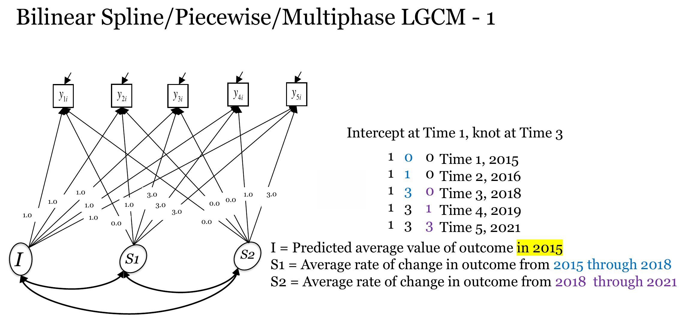{#fig-bilinear1-diagram fig-alt="Path diagram of the bilinear model with the intercept at time 1 and the knot at time 3" width="90%"}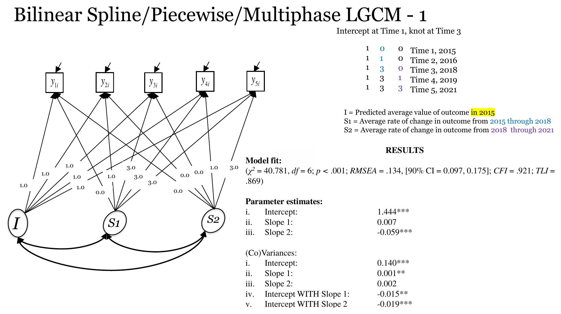{#fig-bilinear1-results fig-alt="Path diagram and Mplus results for version 4.1 of the bilinear model" width="90%"}### Version 4.2: the intercept at the knotIn version 4.2 the early-phase slope has time scores of $-3, -2, 0, 0, 0$, so both slopes are zero in 2018. The intercept factor refers to the predicted average loneliness score in 2018, the year of the knot. Its mean is `r f3(g(fit_bilinear_2, "i", "~1"))` (standard error `r f3(gse(fit_bilinear_2, "i", "~1"))`). It is not a new finding. It equals the prediction of version 4.1 for 2018, namely $`r f3(g(fit_bilinear, "i", "~1"))` + 3 \times `r f3(g(fit_bilinear, "s1", "~1"))` = `r f3(g(fit_bilinear, "i", "~1") + 3 * g(fit_bilinear, "s1", "~1"))`$. The intercept variance is `r f3(g(fit_bilinear_2, "i", "~~", "i"))`, a little smaller than in version 4.1.The covariance of the intercept factor with the early-phase slope is now `r f3(g(fit_bilinear_2, "i", "~~", "s1"))` (*p* = `r fp(gp(fit_bilinear_2, "i", "~~", "s1"))`), whereas it was `r f3(g(fit_bilinear, "i", "~~", "s1"))` in version 4.1. This is not a contradiction. In version 4.1 the covariance describes how the level in 2015 relates to the change from 2015 to 2018. In version 4.2 it describes how the level in 2018 relates to the same change, and a participant who is high in 2018 is partly high because of a positive change before 2018. The sign of an intercept-slope covariance depends on where the intercept is placed, and covariances from differently centered models cannot be compared directly [@biesanz2004coding]. The problem with the late-phase slope remains.@fig-bilinear2-diagram and @fig-bilinear2-results show the slides for this version. The numbers on the results slide agree with the lavaan output.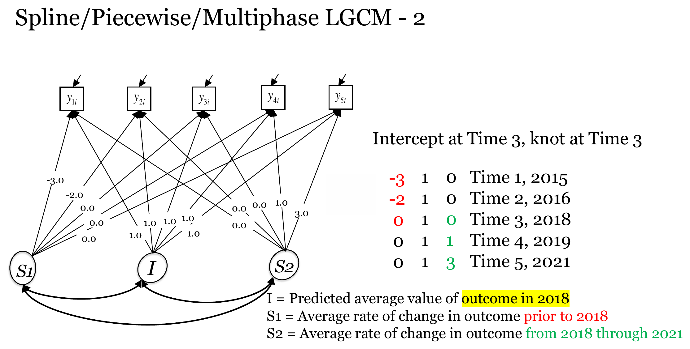{#fig-bilinear2-diagram fig-alt="Path diagram of the spline model with the intercept at time 3 and the knot at time 3" width="90%"}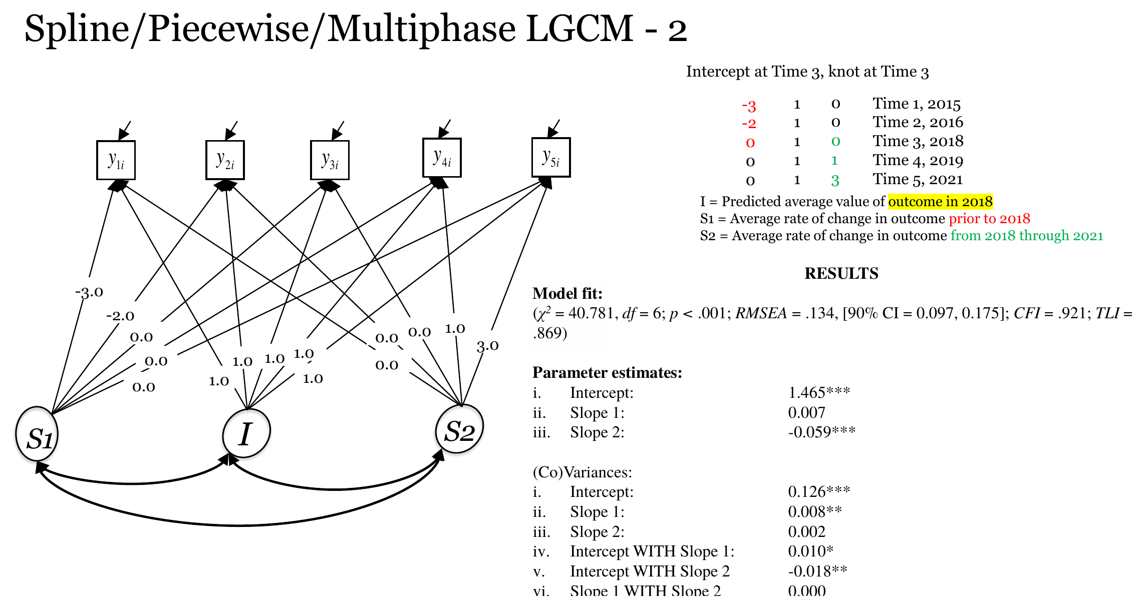{#fig-bilinear2-results fig-alt="Path diagram and Mplus results for version 4.2 of the spline model" width="90%"}### Version 4.3: the intercept at the last waveAt the last wave, in 2021, both slopes are zero in version 4.3, so the intercept factor refers to the predicted average loneliness score at the end of the observation period. Its mean is `r f3(g(fit_bilinear_3, "i", "~1"))` (standard error `r f3(gse(fit_bilinear_3, "i", "~1"))`), which equals $`r f3(g(fit_bilinear, "i", "~1"))` + 3 \times `r f3(g(fit_bilinear, "s1", "~1"))` + 3 \times (`r f3(g(fit_bilinear, "s2", "~1"))`) = `r f3(g(fit_bilinear, "i", "~1") + 3 * g(fit_bilinear, "s1", "~1") + 3 * g(fit_bilinear, "s2", "~1"))`$ from version 4.1.The two slopes carry swapped labels here. The factor `s1` has the time scores $-3, -3, -3, -2, 0$ and is the late-phase slope, with a mean of `r f3(g(fit_bilinear_3, "s1", "~1"))` and a variance of `r f3(g(fit_bilinear_3, "s1", "~~", "s1"))`. The factor `s2` has the time scores $-3, -2, 0, 0, 0$ and is the early-phase slope, with a mean of `r f3(g(fit_bilinear_3, "s2", "~1"))` and a variance of `r f3(g(fit_bilinear_3, "s2", "~~", "s2"))`. These are the same numbers as the ones of `s2` and `s1` in version 4.1. The diagram on the slide for this version (@fig-bilinear3-diagram) labels the slopes the other way round. The estimates on the results slide (@fig-bilinear3-results), for example the slope mean of -0.059 listed as Slope 1, follow the lavaan labeling.The intercept variance in version 4.3 is `r f3(g(fit_bilinear_3, "i", "~~", "i"))` (standard error `r f3(gse(fit_bilinear_3, "i", "~~", "i"))`, *p* = `r fp(gp(fit_bilinear_3, "i", "~~", "i"))`), much smaller than in versions 4.1 and 4.2. It should not be read as a small difference between participants in 2021. It is the variance of the sum of the version 4.1 intercept factor, three times the early-phase slope and three times the late-phase slope. Its value comes from the variances and from the covariances of the three factors, and the covariance of the intercept factor with the late-phase slope is the one that is inadmissible in version 4.1. In version 4.3 the implied correlation between the intercept factor and the late-phase slope (`s1`) is `r f3(cov2cor(lavInspect(fit_bilinear_3, "cov.lv"))["i", "s1"])`, again beyond $-1$. The small variance is therefore an artifact of the improper solution, and the FIML fit below gives a larger value. The covariance of the intercept factor with the early-phase slope is `r f3(g(fit_bilinear_3, "i", "~~", "s2"))` (*p* = `r fp(gp(fit_bilinear_3, "i", "~~", "s2"))`) and with the late-phase slope it is `r f3(g(fit_bilinear_3, "i", "~~", "s1"))` (*p* = `r fp(gp(fit_bilinear_3, "i", "~~", "s1"))`).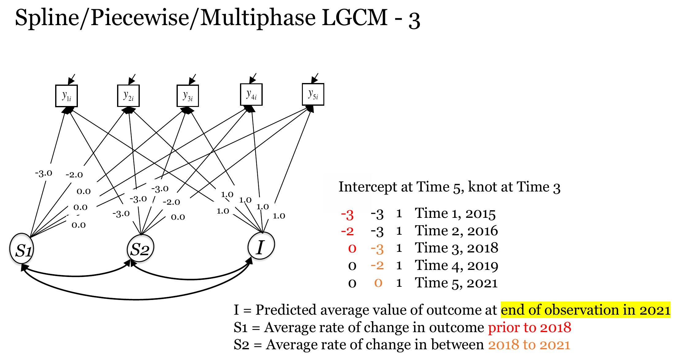{#fig-bilinear3-diagram fig-alt="Path diagram of the spline model with the intercept at time 5 and the knot at time 3" width="90%"}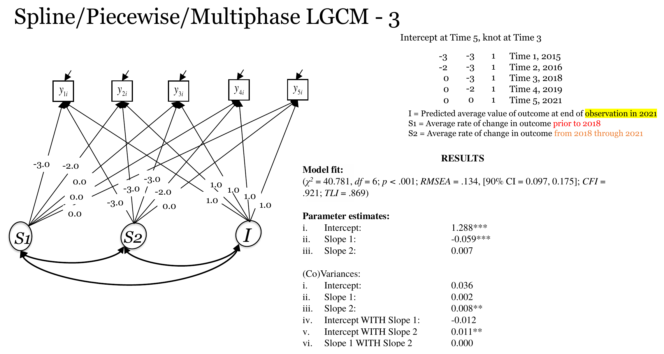{#fig-bilinear3-results fig-alt="Path diagram and Mplus results for version 4.3 of the spline model" width="90%"}::: {.callout-tip title="Where to put the knot and where to put the intercept"}These are two separate decisions. The knot is the point at which the rate of change is allowed to change. It should be based on the design or on theory, and it changes the model and its fit. The point at which the intercept factor is defined is a matter of interpretation, and it does not change the model or its fit. A useful habit is to choose the intercept factor so that the research question can be read from one parameter. If the question is about the level at the end of the study, version 4.3 is the natural choice. If the question is about the level at the knot, use version 4.2.:::## Comparing the bilinear model with the earlier modelsThe first three models are refitted here with the workshop syntax. The chi-square difference test and the information criteria below are an addition to the workshop code, which showed a comparison on a slide (@fig-comparison-slide). The quadratic model gives the same warning about the latent covariance matrix as in @sec-basic.```{r}#| label: refit-earlier-modelsnogrowth <-' i =~ 1*lone1 + 1*lone2 + 1*lone3 + 1*lone4 + 1*lone5'fit_nogrowth <-growth(nogrowth, data = data)linear <-' i =~ 1*lone1 + 1*lone2 + 1*lone3 + 1*lone4 + 1*lone5 s =~ 0*lone1 + 1*lone2 + 3*lone3 + 4*lone4 + 6*lone5'fit_linear <-growth(linear, data = data)quadratic <-' i =~ 1*lone1 + 1*lone2 + 1*lone3 + 1*lone4 + 1*lone5 s =~ 0*lone1 + 1*lone2 + 3*lone3 + 4*lone4 + 6*lone5 q =~ 0*lone1 + 1*lone2 + 9*lone3 + 16*lone4 + 36*lone5'fit_quadratic <-growth(quadratic, data = data)# Addition to the workshop code: chi-square difference test of the linear against the bilinear modellrt <-anova(fit_bilinear, fit_linear)```The no growth, linear and quadratic models of @sec-basic form a sequence of nested models. Each is a restricted version of the next, so the models can be compared with chi-square difference tests [@bentler1980significance]. The linear model is also nested in the bilinear model, because it is the bilinear model with the two slope factors set equal. This restriction removes `r fitMeasures(fit_linear, "df") - fitMeasures(fit_bilinear, "df")` parameters. The chi-square difference is `r f2(lrt[2, "Chisq diff"])` on `r lrt[2, "Df diff"]` degrees of freedom, and the reduced linear model is rejected, so the bilinear model fits better. The restriction puts a variance (that of the difference between the two slopes) on the boundary of its parameter space, so the *p*-value is only approximate [@self1987asymptotic].The bilinear and the quadratic model are not nested in each other. The bilinear model has `r fitMeasures(fit_bilinear, "npar")` parameters and `r fitMeasures(fit_bilinear, "df")` degrees of freedom, exactly like the quadratic model, and neither is a restricted version of the other. The chi-square difference test is then not available, and the two models are compared with the information criteria AIC [@akaike1974new] and BIC [@schwarz1978estimating]. Lower values are better, and the criteria penalize the number of parameters.```{r}#| label: tbl-ic#| tbl-cap: "Information criteria and fit of the models (listwise deletion). This table is an addition to the workshop code."fits <-list(`No growth`= fit_nogrowth, `Linear`= fit_linear, `Quadratic`= fit_quadratic,`Bilinear 4.1`= fit_bilinear, `Bilinear 4.2`= fit_bilinear_2, `Bilinear 4.3`= fit_bilinear_3)ic <-data.frame(Model =names(fits),Parameters =sapply(fits, function(f) fitMeasures(f, "npar")),df =sapply(fits, function(f) fitMeasures(f, "df")),Chisq =sapply(fits, function(f) fitMeasures(f, "chisq")),AIC =sapply(fits, AIC),BIC =sapply(fits, BIC),CFI =sapply(fits, function(f) fitMeasures(f, "cfi")),RMSEA =sapply(fits, function(f) fitMeasures(f, "rmsea")))knitr::kable(ic, digits =3, row.names =FALSE)```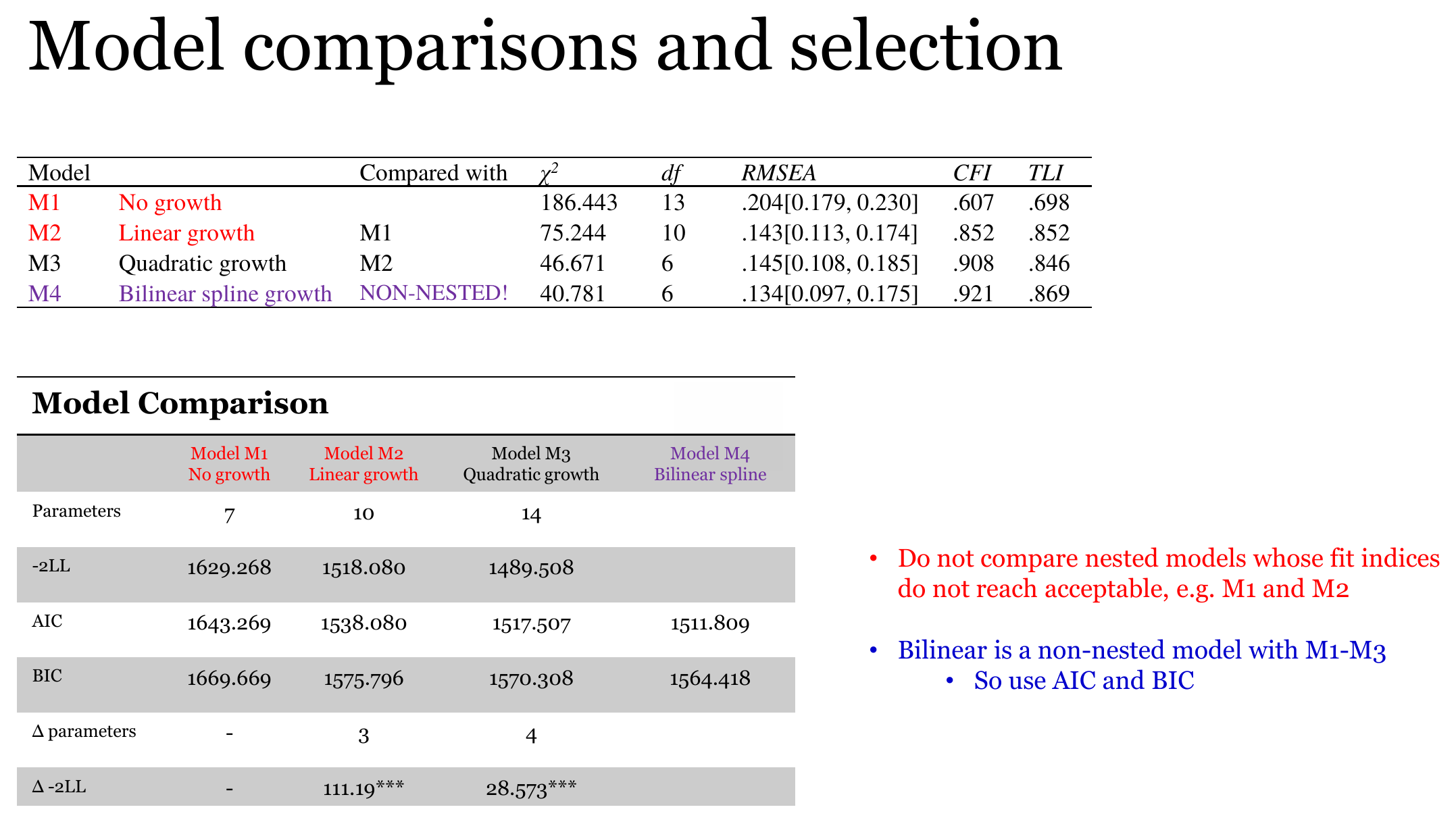{#fig-comparison-slide fig-alt="Table with fit indices and information criteria of the no growth, linear, quadratic and bilinear spline models" width="90%"}The bilinear model has the lowest AIC (`r f3(AIC(fit_bilinear))`) and the lowest BIC (`r f3(BIC(fit_bilinear))`) of the models in the table. The quadratic model has an AIC of `r f3(AIC(fit_quadratic))` and a BIC of `r f3(BIC(fit_quadratic))`. Since both models have the same number of parameters, the penalty terms cancel, and each criterion differs by `r f3(AIC(fit_quadratic) - AIC(fit_bilinear))`, which is the difference between the two deviances. The comparison therefore favors the bilinear model, but the difference is modest. Both models fit poorly by the usual cut-offs and both give the same warning about the latent covariance matrix. The information criteria say which of the models describes the data better. They do not say that the best model fits well. The three versions have identical criteria in the table, as expected for the same model.## A check on the near-zero slope varianceThe warning points to the variance of the late-phase slope. A natural reaction is to fix this variance to zero, which also fixes its covariances to zero, and to treat the late-phase slope as a fixed effect that is the same for every participant. The following code is an addition to the workshop code.```{r}#| label: fix-s2-variance# Addition to the workshop code (not part of the workshop script):# fix the variance of the late-phase slope, and its covariances, to zerobilinear_fixed <-paste(bilinear, "\n s2 ~~ 0*s2 + 0*i + 0*s1")fit_bilinear_fixed <-growth(bilinear_fixed, data = data)round(fitMeasures(fit_bilinear_fixed, c("chisq", "df", "cfi", "tli", "rmsea", "srmr", "aic", "bic")), 3)```The restriction removes `r fitMeasures(fit_bilinear_fixed, "df") - fitMeasures(fit_bilinear, "df")` degrees of freedom. The chi-square increases from `r fmx(fit_bilinear, "chisq")` to `r fmx(fit_bilinear_fixed, "chisq")`, CFI drops from `r fmx(fit_bilinear, "cfi")` to `r fmx(fit_bilinear_fixed, "cfi")` and RMSEA increases to `r fmx(fit_bilinear_fixed, "rmsea")`. The model has no warning anymore, but its fit is worse than that of the unrestricted bilinear model and also worse than that of the linear model (chi-square `r fmx(fit_linear, "chisq")` on `r fitMeasures(fit_linear, "df")` degrees of freedom, AIC `r f3(AIC(fit_linear))`, against `r fmx(fit_bilinear_fixed, "chisq")` on `r fitMeasures(fit_bilinear_fixed, "df")` degrees of freedom and AIC `r f3(AIC(fit_bilinear_fixed))`). Part of the better fit of the unrestricted model may rest on the inadmissible covariance of the intercept factor with the late-phase slope, and these data cannot say more. The likelihood ratio test is not appropriate for a restriction that puts a variance at its boundary [@self1987asymptotic], so we use the change in fit only descriptively.Fixing the variance is therefore not a remedy here. The options are to report the original model with a clear description of the problem, to use a design with more waves in each phase so that each slope is based on more than three points, or to look for a different description of the change. Each phase here rests on only three waves, and the knot is shared by both phases. This limits how much information there is about the variance of each slope.## Sensitivity to the missing data handlingThe results above use the participants with complete data on loneliness. As a check, which is an addition to the workshop, the three versions are refitted with full information maximum likelihood (FIML), which uses all available scores (see @sec-prelims). lavaan ignores the rows without any loneliness score, so that `r lavInspect(growth(bilinear, data = data, missing = "fiml"), "ntotal")` participants contribute.```{r}#| label: fiml-sensitivity# Addition to the workshop code: FIML sensitivity analysisfit_bilinear_fiml <-growth(bilinear, data = data, missing ="fiml")fit_bilinear_2_fiml <-growth(bilinear_2, data = data, missing ="fiml")fit_bilinear_3_fiml <-growth(bilinear_3, data = data, missing ="fiml")sens <-data.frame(Parameter =c("Intercept mean", "Early-phase slope mean", "Late-phase slope mean","Intercept variance", "Early-phase slope variance", "Late-phase slope variance"),Listwise =c(g(fit_bilinear, "i", "~1"), g(fit_bilinear, "s1", "~1"), g(fit_bilinear, "s2", "~1"),g(fit_bilinear, "i", "~~", "i"), g(fit_bilinear, "s1", "~~", "s1"), g(fit_bilinear, "s2", "~~", "s2")),FIML =c(g(fit_bilinear_fiml, "i", "~1"), g(fit_bilinear_fiml, "s1", "~1"), g(fit_bilinear_fiml, "s2", "~1"),g(fit_bilinear_fiml, "i", "~~", "i"), g(fit_bilinear_fiml, "s1", "~~", "s1"), g(fit_bilinear_fiml, "s2", "~~", "s2")))knitr::kable(sens, digits =3)round(fitMeasures(fit_bilinear_fiml, c("chisq", "df", "cfi", "tli", "rmsea", "srmr")), 3)# smallest eigenvalue of the latent covariance matrix under FIMLsapply(list(`4.1`= fit_bilinear_fiml, `4.2`= fit_bilinear_2_fiml, `4.3`= fit_bilinear_3_fiml),function(f) min(eigen(lavInspect(f, "cov.lv"))$values))```The means of the growth factors change little. The intercept factor of version 4.1 has a mean of `r f3(g(fit_bilinear_fiml, "i", "~1"))` under FIML (`r f3(g(fit_bilinear, "i", "~1"))` with listwise deletion), the early-phase slope has a mean of `r f3(g(fit_bilinear_fiml, "s1", "~1"))` (`r f3(g(fit_bilinear, "s1", "~1"))`) and the late-phase slope has a mean of `r f3(g(fit_bilinear_fiml, "s2", "~1"))` (`r f3(g(fit_bilinear, "s2", "~1"))`). The variances are somewhat larger. The variance of the late-phase slope goes from `r f3(g(fit_bilinear, "s2", "~~", "s2"))` to `r f3(g(fit_bilinear_fiml, "s2", "~~", "s2"))` (*p* = `r fp(gp(fit_bilinear_fiml, "s2", "~~", "s2"))`), so it remains small and not distinguishable from zero. In version 4.3 the intercept variance is `r f3(g(fit_bilinear_3_fiml, "i", "~~", "i"))` under FIML (standard error `r f3(gse(fit_bilinear_3_fiml, "i", "~~", "i"))`), against `r f3(g(fit_bilinear_3, "i", "~~", "i"))` with listwise deletion. The smallest eigenvalue of the latent covariance matrix is positive in all three FIML fits, so the warning does not appear. The chi-square values of the two analyses are not compared, since they are based on different numbers of participants.A second check changes the estimator. FIML with the robust maximum likelihood estimator `MLR`[@yuan2000three] gives the following fit for version 4.1.```{r}#| label: mlr-sensitivity# Addition to the workshop code: FIML with a robust estimatorfit_bilinear_mlr <-growth(bilinear, data = data, missing ="fiml", estimator ="MLR")round(fitMeasures(fit_bilinear_mlr, c("chisq.scaled", "df.scaled", "cfi.robust", "rmsea.robust")), 3)```The scaled chi-square is `r fmx(fit_bilinear_mlr, "chisq.scaled")`, compared with `r fmx(fit_bilinear_fiml, "chisq")` for the FIML fit with the standard chi-square on the same participants. The robust CFI is `r fmx(fit_bilinear_mlr, "cfi.robust")` and the robust RMSEA is `r fmx(fit_bilinear_mlr, "rmsea.robust")`. The smaller scaled statistic is what is expected with skewed scores (see @sec-prelims).## What changed compared with the previous modelThe quadratic model of @sec-basic and the bilinear model have the same number of parameters and the same degrees of freedom. The difference lies in the shape of the average trajectory. The quadratic model describes one smooth curve and the bilinear model describes two straight pieces with a bend at the knot. The chi-square drops from `r fmx(fit_quadratic, "chisq")` to `r fmx(fit_bilinear, "chisq")`, and the information criteria favor the bilinear model slightly. Compared with the linear model, the bilinear model allows the average rate of change to differ between the two phases and adds a second slope factor, with its variance and covariances. The bilinear model fits better than the linear model, but the data do not show whether this comes from the different means of the two phases, from the extra slope factor, or from the inadmissible solution. The extra slope factor is also the source of the warning, because it has to be estimated from three waves.## What this model answers and what it cannot tellThe model answers whether the average rate of change differs between the two phases and whether participants differ in the rate of change in each phase, given a knot that the researcher has chosen. For this dataset and the knot at the third wave, the average rate before the knot is small and the average rate after it is negative. Participants differ in the starting level and, slightly, in the early-phase rate, but the data do not settle whether they differ in the late-phase rate.The model does not tell why the rate of change differs between the phases, and it does not tell that anything happens at the knot. The knot at the third wave was fixed in advance, and other knot positions were not compared. With only five waves, the choices for the knot are few. The fit is poor by the usual cut-offs, so the model does not describe the covariance structure of the five waves well. The non-positive definite covariance matrix means that the variance and covariance estimates involving the late-phase slope are not reliable. The three versions of the model cannot be told apart by fit, so the choice among them is a choice of interpretation and not a result.## Researcher's perspectiveThe location of the knot should be motivated before the analysis, by the design or by theory, and it should be stated in the report as a choice. If several knot locations are tried, say so, since trying many and reporting the best one overstates the evidence.Because the three versions have the same fit, choose the version in which the parameter of interest is in the intercept factor, and say where the intercept factor is located. When intercept-slope covariances are reported, state the point in time to which they refer, since the sign can change with the centering. If you compare your results with the literature, check how time was coded there.A warning about the latent covariance matrix is part of the results and should be reported with the variance estimate that causes it, together with what was done about it. Here the near-zero variance of the late-phase slope prevents strong statements about individual differences in that phase. Fixing the variance to zero made the fit worse, and the FIML analysis removed the warning. Both facts belong in the write-up. Report that listwise deletion was used, give the number of participants analyzed, and give the FIML result as a check (@sec-prelims).The next chapter adds a second variable that is measured at every wave, a time-varying covariate (@sec-tvc).