4 Time-varying covariates
In Chapter 2 and Chapter 3 we asked about the shape of the average trajectory of loneliness. Every model so far described one outcome measured five times, and the only explanatory variable was time itself. In this chapter we add a second variable that is also measured at each wave, hostility (host1 to host5), and we ask whether it goes together with loneliness at the same wave. The growth part of the model stays the linear growth model. What is new is the set of paths from hostility to loneliness.
4.1 Why this model
A linear growth model describes where each person starts and how fast the person changes, but it says nothing about wave-specific departures from that path. A person may score above their own trajectory at one wave and below it at another. A time-varying covariate (TVC) is a variable with its own value at every wave that may help to account for such departures. This is the question the model answers: does the score on hostility at a given wave go together with the score on loneliness at that same wave, once the growth trajectory is in the model?
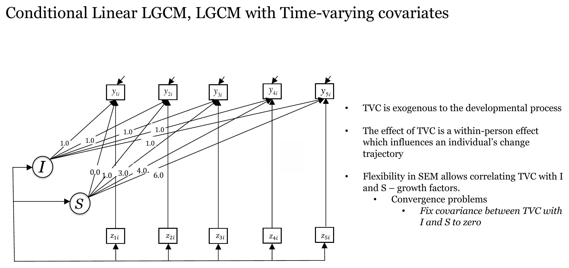
Time-varying covariates differ from the time-invariant covariates of Chapter 5, which are measured once and can only be related to the growth factors. A TVC is related to the outcome at each wave, so it can be tied to the wave-specific scores. In the workshop this model was introduced as a conditional linear growth model with time-varying covariates, and the slide in Figure 4.1 summarizes the ideas we use below.
4.2 The idea in plain language
The covariate is treated as exogenous. This means that hostility is taken as given. The model uses it to predict loneliness, but nothing in the model predicts hostility, and the model does not describe how hostility itself changes over time. The measurements of hostility are allowed to have their own means, variances and covariances, and that is all. As a consequence, the model cannot say whether hostility comes before loneliness, after it, or neither.
The paths run from hostility at wave \(t\) to loneliness at the same wave \(t\). Each path is a regression of the wave-specific loneliness score on the wave-specific hostility score, and in the workshop code the five paths are estimated separately. Because the growth factors take care of the average trend and the individual differences in level and rate of change, the paths are meant to capture the association with the departures from the trajectory. The slide calls this a within-person effect. This reading holds only to the extent that the stable differences in hostility between persons are unrelated to the growth factors, which this model assumes through its syntax and does not test. The separation of within-person and between-person effects is discussed by Curran & Bauer (2011).
The growth factors now have a different meaning. In the linear model the intercept factor was the expected loneliness at wave 1. Here it is the expected loneliness at wave 1 for a person whose hostility score at wave 1 is zero. The slope factor is the average rate of change in the part of loneliness that is not accounted for by hostility. This changes how the growth means are read.
4.3 A concrete example
We use the same dataset as before. At each of the five waves (2015, 2016, 2018, 2019 and 2021) participants have a score on loneliness and a score on hostility. The time scores remain 0, 1, 3, 4 and 6, with one unit equal to one year and the year 2015 as time 0. In the dataset the minimum is 1.0 at every wave and the maximum lies between 4.5 and 5.0. A score of zero on hostility therefore does not occur in the dataset, and this fact matters for the interpretation of the intercept.
The distribution of hostility is skewed to the right, as the distribution of loneliness is. The skewness of the five hostility scores ranges from 1.67 to 3.16, and their kurtosis from 2.85 to 12.58. Most participants score low, and a few score high. The consequences of this for the maximum likelihood estimator are described in Chapter 1.
4.4 The formal model
For person \(i\) at wave \(t\), loneliness is written as
\[ \text{lone}_{ti} = \eta_{0i} + \lambda_t \, \eta_{1i} + \beta_t \, \text{host}_{ti} + \varepsilon_{ti}, \]
with time scores \(\lambda_t = 0, 1, 3, 4, 6\) and growth factors \(\eta_{0i} = \mu_0 + \zeta_{0i}\) and \(\eta_{1i} = \mu_1 + \zeta_{1i}\). The only new term is \(\beta_t \, \text{host}_{ti}\). The coefficient has the subscript \(t\) because the five paths are freely estimated and no equality constraint is placed on them.
Hostility is part of the model as a random variable with a mean \(\mu_{h,t}\) at each wave and with variances and covariances among the five waves. The covariances of hostility with the growth factors \(\eta_0\) and \(\eta_1\) are not estimated and are therefore zero in the model. Taking expectations gives the equation that we need for interpretation:
\[ E(\text{lone}_t) = \mu_0 + \lambda_t \, \mu_1 + \beta_t \, \mu_{h,t}. \]
The expected loneliness at each wave is the sum of a growth part and a hostility part. When hostility is part of the model, the growth means \(\mu_0\) and \(\mu_1\) describe only the first part.
4.5 R implementation
The model below is the workshop code and is not changed. It has three parts. The first part is the linear growth model, as before. The second part holds the five regressions of loneliness on hostility, and the third part estimates the means of the hostility scores and the covariances among them.
Code
timevaryingcov <- ' i =~ 1*lone1 + 1*lone2 + 1*lone3 + 1*lone4 + 1*lone5
                    s =~ 0*lone1 + 1*lone2 + 3*lone3 + 4*lone4 + 6*lone5
# Time-varying covariates
lone1 ~ host1             #lone1 ~ eq*host1
lone2 ~ host2             #lone2 ~ eq*host2
lone3 ~ host3             #lone3 ~ eq*host3
lone4 ~ host4             #lone4 ~ eq*host4
lone5 ~ host5             #lone5 ~ eq*host5

#Estimate the means of the TVC
host1 ~ 1
host2 ~ 1
host3 ~ 1
host4 ~ 1
host5 ~ 1

#Estimate covariance between TVC
host1 ~~ host2 + host3 + host4 + host5
host2 ~~ host3 + host4 + host5
host3 ~~ host4 + host5
host4 ~~ host5'

fit_timevaryingcov <- growth(timevaryingcov, data = data)
summary(fit_timevaryingcov, fit.measures = TRUE)
lavaan 0.6.17 ended normally after 109 iterations
Estimator ML
Optimization method NLMINB
Number of model parameters 35
Used Total
Number of observations 321 442
Model Test User Model:
Test statistic 103.191
Degrees of freedom 30
P-value (Chi-square) 0.000
Model Test Baseline Model:
Test statistic 2956.213
Degrees of freedom 45
P-value 0.000
User Model versus Baseline Model:
Comparative Fit Index (CFI) 0.975
Tucker-Lewis Index (TLI) 0.962
Loglikelihood and Information Criteria:
Loglikelihood user model (H0) -659.170
Loglikelihood unrestricted model (H1) -607.575
Akaike (AIC) 1388.340
Bayesian (BIC) 1520.341
Sample-size adjusted Bayesian (SABIC) 1409.326
Root Mean Square Error of Approximation:
RMSEA 0.087
90 Percent confidence interval - lower 0.069
90 Percent confidence interval - upper 0.106
P-value H_0: RMSEA <= 0.050 0.001
P-value H_0: RMSEA >= 0.080 0.755
Standardized Root Mean Square Residual:
SRMR 0.059
Parameter Estimates:
Standard errors Standard
Information Expected
Information saturated (h1) model Structured
Latent Variables:
Estimate Std.Err z-value P(>|z|)
i =~
lone1 1.000
lone2 1.000
lone3 1.000
lone4 1.000
lone5 1.000
s =~
lone1 0.000
lone2 1.000
lone3 3.000
lone4 4.000
lone5 6.000
Regressions:
Estimate Std.Err z-value P(>|z|)
lone1 ~
host1 0.719 0.017 41.813 0.000
lone2 ~
host2 0.722 0.014 52.466 0.000
lone3 ~
host3 0.738 0.012 63.080 0.000
lone4 ~
host4 0.735 0.015 48.645 0.000
lone5 ~
host5 0.737 0.022 33.693 0.000
Covariances:
Estimate Std.Err z-value P(>|z|)
host1 ~~
host2 0.161 0.018 8.703 0.000
host3 0.105 0.018 5.860 0.000
host4 0.053 0.013 4.153 0.000
host5 0.036 0.011 3.452 0.001
host2 ~~
host3 0.158 0.021 7.358 0.000
host4 0.079 0.015 5.286 0.000
host5 0.052 0.012 4.247 0.000
host3 ~~
host4 0.120 0.016 7.325 0.000
host5 0.069 0.013 5.280 0.000
host4 ~~
host5 0.064 0.010 6.527 0.000
i ~~
s -0.003 0.001 -4.609 0.000
Intercepts:
Estimate Std.Err z-value P(>|z|)
host1 1.432 0.028 51.297 0.000
host2 1.459 0.032 45.207 0.000
host3 1.535 0.034 45.422 0.000
host4 1.311 0.025 52.956 0.000
host5 1.294 0.021 62.524 0.000
i 0.414 0.026 15.690 0.000
s -0.010 0.007 -1.399 0.162
Variances:
Estimate Std.Err z-value P(>|z|)
.lone1 0.024 0.003 7.834 0.000
.lone2 0.025 0.003 9.540 0.000
.lone3 0.038 0.003 11.346 0.000
.lone4 0.031 0.003 10.917 0.000
.lone5 0.017 0.003 5.695 0.000
host1 0.250 0.020 12.669 0.000
host2 0.334 0.026 12.669 0.000
host3 0.367 0.029 12.669 0.000
host4 0.197 0.016 12.669 0.000
host5 0.138 0.011 12.669 0.000
i 0.028 0.003 8.206 0.000
s 0.001 0.000 4.757 0.0004.5.1 Reading the syntax
The five lines lone_t ~ host_t carry no label, so each coefficient is free. The commented text beside each line (eq*) shows how the same coefficient could be held equal across waves, by giving the five paths one common label. That version is not used in the workshop. Here the association is allowed to differ from wave to wave, and the model can then show whether it does. The paths are the regression weights that the slide draws as the vertical arrows from the covariates to the outcomes.
The lines host1 ~ 1 and so on make the means of the covariates parameters of the model, and the output lists them among the intercepts. The covariates are treated as random variables with estimated means, variances and covariances, and not as fixed values. In growth() the intercepts of the observed loneliness scores are fixed to zero, which is why the output shows no intercepts for lone1 to lone5. All the mean structure of loneliness therefore passes through the intercept factor, the slope factor and the hostility terms, as in the expectation equation above.
The lines host1 ~~ host2 + ... estimate the ten covariances among the five hostility scores. Hostility is measured repeatedly in the same persons, so the scores are expected to be related across waves. These covariances let the model describe this dependence without saying anything about its direction. This is also what exogeneity means in practice. The covariate may be correlated with itself over time, but it is not explained by earlier loneliness or by earlier hostility.
The syntax contains no statement of the type i ~~ host1 or s ~~ host1. The slide in Figure 4.1 says that structural equation modeling allows the covariates to be correlated with the intercept and slope factors, and that these covariances can be fixed to zero when there are convergence problems. In this syntax such covariances are not added, and the parameter table (parTable(fit_timevaryingcov)) shows no parameter that links hostility with i or s. The model thus sets these ten covariances to zero. This is the option that the slide offers as a remedy for convergence problems, and here it is simply what the default does. The only covariance among the latent variables that is estimated is the one between the intercept factor and the slope factor, which lavaan adds by default for the two exogenous growth factors. The consequence for the interpretation is examined in Section 4.9.
4.6 Understanding the output
4.6.1 Missing data and sample size
The output reports 321 used observations out of 442 rows, because growth() was called with its default settings, which means listwise deletion (see Chapter 1). The number of participants with complete scores on loneliness and hostility is 321, which equals the number with complete loneliness scores alone (321). Hostility is also incompletely observed in the full dataset, with between 390 and 413 observed scores per wave, but adding it does not reduce the number used any further. The results below describe the 321 participants with complete data, and the sensitivity analysis later in the chapter uses all participants. The estimation converged (lavInspect(fit, "converged") returns TRUE) and lavaan printed no warning for this model. The covariance matrix of the latent variables is positive definite, although its smallest eigenvalue (0.0005) is close to zero.
4.6.2 Model fit
The test statistic is \(\chi^2(30) = 103.19\), \(p < .001\). The exact fit is rejected. The approximate indices are more favorable: CFI is 0.975, TLI is 0.962, RMSEA is 0.087 with a 90% confidence interval from 0.069 to 0.106, and SRMR is 0.059. The CFI, TLI and SRMR are in the range that is usually regarded as good (Hu & Bentler, 1999). The RMSEA is borderline. Its confidence interval does not exclude values above .08, and the test of close fit (RMSEA at most .05) is rejected (\(p = 0.001\)). The CFI is therefore high and the RMSEA is borderline. The cut-offs of Hu & Bentler (1999) are guidance and not fixed boundaries.
The indices cannot be compared directly with those of the linear growth model (CFI 0.852, RMSEA 0.143). The linear model involves five observed variables and this model involves ten. The means, variances and covariances of the five hostility scores are freely estimated, so that part of the data is reproduced exactly. The baseline model, against which CFI and TLI are computed, has a chi-square of 2956.2 on 45 degrees of freedom here, against 451.2 on 10 for the linear model, because the five hostility scores are strongly related to each other and to loneliness. A large baseline chi-square tends to give a higher CFI for the same amount of misfit, so the CFI of this model should be read with that in mind. The RMSEA does not depend on the baseline model. The chi-square, the AIC (Akaike, 1974) and the BIC (Schwarz, 1978) of the two models are also not comparable, because they are computed for different sets of variables. What can be said is that the paths from hostility reduce the residual variances of loneliness, as shown below.
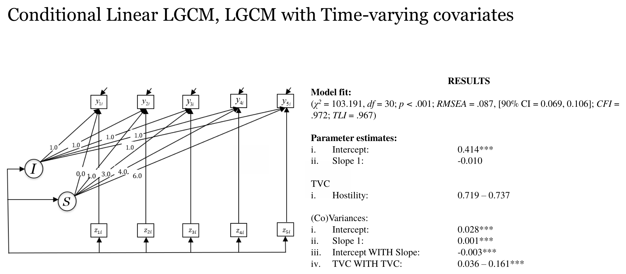
The slide with the results is shown in Figure 4.2. It was produced with Mplus. The chi-square, the RMSEA and its interval, and the parameter estimates agree with the lavaan output used in this chapter, except that the range of the hostility paths on the slide ends at 0.737, whereas the path at wave 3 is 0.738 in the R output. The CFI (.972) and TLI (.967) on the slide differ slightly from the lavaan values reported above (0.975 and 0.962). We use the R output throughout.
4.6.3 The effect of hostility on loneliness
Table 4.1 gives the five regression coefficients. They are close to each other, from 0.719 to 0.738, although nothing in the syntax forced them to be similar. All five are clearly different from zero. The standardized coefficients range from 0.812 to 0.885.
Code
tab_paths <- data.frame(
  Wave = 1:5,
  Estimate = f3(paths$est),
  SE = f3(paths$se),
  z = f2(paths$z),
  Standardized = f3(paths_std$est.std)
)
knitr::kable(tab_paths, align = "lrrrr")| Wave | Estimate | SE | z | Standardized |
|---|---|---|---|---|
| 1 | 0.719 | 0.017 | 41.81 | 0.846 |
| 2 | 0.722 | 0.014 | 52.47 | 0.885 |
| 3 | 0.738 | 0.012 | 63.08 | 0.883 |
| 4 | 0.735 | 0.015 | 48.64 | 0.826 |
| 5 | 0.737 | 0.022 | 33.69 | 0.812 |
The association is strong in this dataset. The proportion of variance in the loneliness scores that is accounted for by the model (the growth factors and hostility together) lies between 0.80 and 0.89 across the waves. The raw correlation between loneliness and hostility at wave 1 in the 321 participants is 0.86, and at wave 3 it is 0.87. The correlation between loneliness at wave 1 and hostility at wave 3 is only 0.40. The association is thus much stronger within a wave than across waves. Correlations this high between two scores from the same wave suggest that the two measures overlap strongly and may be close to redundant in this dataset. The data cannot tell what the two measures share.
Because the paths are close to each other, one may be tempted to hold them equal. That is a model comparison that the workshop does not run, and the commented eq* labels show only where it would be done. Whether the equality constraint is acceptable would need to be tested and not assumed.
4.6.4 Hostility on its own
The means of hostility in the 321 participants are 1.432, 1.459, 1.535, 1.311, 1.294 for waves 1 to 5. They rise slightly up to wave 3 and are lower at waves 4 and 5. The variances of the hostility scores are between 0.138 and 0.367.
The ten covariances among the hostility scores are all positive and clearly different from zero. The largest is between waves 1 and 2 (0.161), and the smallest between waves 1 and 5 (0.036). Covariances between measurements that are further apart in time tend to be smaller, which is the usual pattern for a variable with some stability that fades over longer intervals. The scale of the covariances depends on the variances, so we only read the pattern and not the size.
4.6.5 The growth factors
The mean of the intercept factor is 0.414 (\(SE = 0.026\)) and the mean of the slope factor is -0.010 (\(SE = 0.007\), \(p = 0.162\)). The variance of the intercept is 0.028 and the variance of the slope is 0.001. Both variances are different from zero, so individual differences remain in both growth factors after hostility is accounted for. The variance of the slope is small in absolute size, as in the linear model, and the covariance between the intercept and the slope is -0.003, which is negative. In the linear model the intercept variance was 0.139 and the slope variance was 0.003. Both are smaller now, which is consistent with part of the variation in loneliness being shared with hostility.
The residual variances of loneliness at the five waves are 0.024, 0.025, 0.038, 0.031, 0.017. In the linear model they were 0.059, 0.114, 0.172, 0.114, 0.047. For wave 3, for example, the value falls from 0.172 to 0.038. The residual variances are smaller when the paths are included, which is consistent with hostility accounting for part of the wave-specific variation that the linear model left as residual.
4.7 Interpretation
4.7.1 What the growth means now say
In the linear model the intercept mean was 1.466 and the slope mean was -0.025. In this model the intercept mean falls to 0.414 and the slope mean to -0.010, a value that is not statistically different from zero when the 321 complete cases are used. These changes follow from the meaning of the growth factors in a model with a covariate, and not from a change in loneliness itself.
Reading the intercept
The intercept factor is now the expected loneliness at wave 1 for a person with a hostility score of zero at wave 1. The observed minimum of hostility is 1.0 at every wave. A hostility score of zero is therefore outside the observed range of the covariate, and the intercept mean of 0.414 is an extrapolation. It is not the typical loneliness at wave 1 of any participant in the dataset. The expected loneliness at wave 1 for a person with the average hostility is obtained by adding the hostility part.
At the mean of hostility at wave 1, the expected loneliness at wave 1 is \(0.414 + 0.719 \times 1.432 = 1.443\). This equals the observed mean of loneliness at wave 1 in these participants (1.443). In the linear model the intercept mean (1.466) was the expected loneliness at wave 1, and it is of the same size as this value. The fall from 1.466 to 0.414 is thus not a sign that loneliness at wave 1 is lower. It reflects a change in what the number refers to.
A similar argument applies to the slope. The model-implied average loneliness at each wave is the sum of the growth part and the hostility part. Table 4.2 shows these values next to the observed means. The change in the average loneliness between wave 1 and wave 5 is -0.136 in the model. Of this, the growth part contributes \(6 \times -0.010 = -0.061\) and the hostility part contributes \(0.737 \times 1.294 - 0.719 \times 1.432 = -0.075\). The average hostility is lower at wave 5 than at wave 1, and because the paths from hostility to loneliness are positive, a part of the average decline in loneliness is carried by the decline in hostility. This is an accounting of the mean structure of the model. It does not show that a decline in hostility produces a decline in loneliness.
Code
tab_means <- data.frame(
  Wave = 1:5,
  Time = c(0, 1, 3, 4, 6),
  Observed = f3(obs_lone),
  Linear = f3(imp_lin),
  `With hostility` = f3(imp_tvc),
  `Hostility part` = f3(hostpart),
  check.names = FALSE
)
knitr::kable(tab_means, align = "rrrrrr")| Wave | Time | Observed | Linear | With hostility | Hostility part |
|---|---|---|---|---|---|
| 1 | 0 | 1.443 | 1.466 | 1.443 | 1.029 |
| 2 | 1 | 1.455 | 1.441 | 1.456 | 1.053 |
| 3 | 3 | 1.523 | 1.391 | 1.517 | 1.133 |
| 4 | 4 | 1.333 | 1.367 | 1.336 | 0.963 |
| 5 | 6 | 1.307 | 1.317 | 1.307 | 0.954 |
4.7.2 How the result can be reported
Across the five waves, a higher hostility score at a given wave goes together with a higher loneliness score at the same wave, with unstandardized coefficients between 0.719 and 0.738. The size of the association is similar at the five waves. After the wave-specific associations with hostility are included, the average linear change in the remaining part of loneliness is small (-0.010 per year) and is not distinguishable from zero in the complete-case analysis, while the participants still differ in their intercepts and slopes. We should also state that the intercept refers to a hostility score of zero.
Same-wave association
Each path links two scores measured at the same wave. The model has no lagged effects and no paths from loneliness to hostility, so it cannot separate a situation in which hostility goes with higher loneliness from one in which loneliness goes with higher hostility, or one in which both are linked to something else. The word “effect” in the output is a label for the regression path and not a causal finding.
4.8 Sensitivity to the missing data handling
The results above are based on 321 of 442 participants. As a check that was not part of the workshop, the model was fitted with full information maximum likelihood (FIML), which uses every participant with at least one observed score (see Chapter 1 for FIML and the missing at random assumption). FIML was found to perform better than listwise deletion in the conditions examined by Enders & Bandalos (2001). Table 4.3 compares the two sets of estimates.
Code
est <- read.csv("data/diag/estimates_listwise_vs_fiml.csv")
est <- est[est$label == "005_timevaryingcov", ]
pick <- function(lhs, op, rhs) est[est$lhs == lhs & est$op == op & est$rhs == rhs, ]
rows <- list(
  c("Path host1 to lone1", "lone1", "~", "host1"),
  c("Path host3 to lone3", "lone3", "~", "host3"),
  c("Path host5 to lone5", "lone5", "~", "host5"),
  c("Intercept mean", "i", "~1", ""),
  c("Slope mean", "s", "~1", ""),
  c("Intercept variance", "i", "~~", "i"),
  c("Slope variance", "s", "~~", "s"),
  c("Variance of host1", "host1", "~~", "host1"),
  c("Variance of host4", "host4", "~~", "host4")
)
tab_fiml <- do.call(rbind, lapply(rows, function(r) {
  p <- pick(r[2], r[3], r[4])
  data.frame(Parameter = r[1], Listwise = f3(p$est_lw), `SE listwise` = f3(p$se_lw),
             FIML = f3(p$est_fiml), `SE FIML` = f3(p$se_fiml), check.names = FALSE)
}))
knitr::kable(tab_fiml, align = "lrrrr")
fiml_s <- pick("s", "~1", "")
fiml_i <- pick("i", "~1", "")
z_fiml_s <- fiml_s$est_fiml / fiml_s$se_fiml
p_fiml_s <- 2 * pnorm(-abs(z_fiml_s))
paths_fiml <- est[est$op == "~" & est$lhs %in% lone_vars, "est_fiml"]| Parameter | Listwise | SE listwise | FIML | SE FIML |
|---|---|---|---|---|
| Path host1 to lone1 | 0.719 | 0.017 | 0.705 | 0.015 |
| Path host3 to lone3 | 0.738 | 0.012 | 0.737 | 0.011 |
| Path host5 to lone5 | 0.737 | 0.022 | 0.739 | 0.018 |
| Intercept mean | 0.414 | 0.026 | 0.427 | 0.024 |
| Slope mean | -0.010 | 0.007 | -0.013 | 0.006 |
| Intercept variance | 0.028 | 0.003 | 0.032 | 0.003 |
| Slope variance | 0.001 | 0.000 | 0.001 | 0.000 |
| Variance of host1 | 0.250 | 0.020 | 0.306 | 0.022 |
| Variance of host4 | 0.197 | 0.016 | 0.266 | 0.019 |
The fit under FIML is similar to the fit under listwise deletion: CFI is 0.977, RMSEA is 0.081 and SRMR is 0.069 for 436 participants. With the robust maximum likelihood estimator (MLR), which corrects the test statistic for non-normality (Yuan & Bentler, 2000), the CFI is 0.982 and the RMSEA is 0.074. The pattern of a high CFI and a borderline RMSEA is the same under FIML and under MLR.
The five paths from hostility to loneliness range from 0.705 to 0.739 under FIML, which is almost the same as the listwise result. The intercept mean is 0.427 and the slope mean is -0.013. The variances of the growth factors are somewhat larger, and so are the variances of the hostility scores, which are noticeably larger at some waves.
There is one result that does not carry over. Under FIML the slope mean is -0.013 with a standard error of 0.006, which gives \(z = -2.10\) and \(p = 0.036\). The slope mean is thus about two standard errors below zero, whereas in the complete-case analysis it was not distinguishable from zero. The slope mean is small in both analyses, and we should not make much of the difference. It does mean that the statement that no average change remains once hostility is included is not stable across the two ways of handling the missing data.
4.9 Two checks that were not part of the workshop
The workshop code does not include the code in this section. The checks are added here because both points affect how the output of the model is read.
4.9.1 Covariances between hostility and the growth factors
We saw that the model sets the covariances between the hostility scores and the two growth factors to zero. The code below frees them, by adding the ten covariances to the workshop syntax. The model is then a less restricted version of the same model, and the two can be compared with a chi-square difference test (Bentler & Bonett, 1980).
Code
# ADDITION, not part of the workshop code: free the covariances of the
# time-varying covariates with the growth factors
timevaryingcov_cov <- paste(timevaryingcov,
  "i ~~ host1 + host2 + host3 + host4 + host5",
  "s ~~ host1 + host2 + host3 + host4 + host5", sep = "\n")
fit_tvc_cov <- growth(timevaryingcov_cov, data = data)
lavTestLRT(fit_timevaryingcov, fit_tvc_cov)
Chi-Squared Difference Test

                   Df    AIC    BIC   Chisq Chisq diff   RMSEA Df diff
fit_tvc_cov        20 1364.4 1534.2  59.292
fit_timevaryingcov 30 1388.3 1520.3 103.191     43.898 0.10276      10
                   Pr(>Chisq)
fit_tvc_cov
fit_timevaryingcov  3.433e-06 ***
---
Signif. codes:  0 '***' 0.001 '**' 0.01 '*' 0.05 '.' 0.1 ' ' 1
The less restricted model converged without a warning. It has 20 degrees of freedom, and the fit is better than that of the workshop model: \(\chi^2 = 59.29\), CFI is 0.987, RMSEA is 0.078 and SRMR is 0.017. The difference in chi-square is 43.90 on 10 degrees of freedom, \(p < .001\). In words, the reduced model is rejected, so the model with the free covariances fits better. Of the five covariances with the intercept, 4 are different from zero at the .05 level, all of them positive (from 0.009 to 0.031). The covariances with the slope are small and negative, and 2 of the five are different from zero at that level. In this dataset, higher hostility at several waves goes together with a higher intercept, which is the part of loneliness at wave 1 that is not accounted for by hostility at wave 1. The intercept mean is 0.453 and the slope mean is -0.012 in this version, so the interpretation of the growth means does not change.
This check is a reminder of the qualification we made about the within-person reading. The model of the workshop assumes that persons with a higher level of hostility in general do not differ in their growth factors. The data are not fully consistent with that assumption, and the paths from hostility should therefore not be seen as purely within-person coefficients. A formal separation of the within-person and the between-person part of the covariate is a different specification (Curran & Bauer, 2011). We make no claim here about how much the paths would change. The test is also based on ten additional parameters, so the individual p values should be read with caution.
4.9.2 Where the intercept points
We said that a hostility score of zero is outside the observed range. A simple remedy is to center hostility before fitting the model, so that the intercept refers to a value that exists in the data. The code below subtracts one common constant, the pooled mean of the hostility scores, from all five hostility variables and fits the workshop model unchanged to the centered data.
Code
# ADDITION, not part of the workshop code: center the hostility scores at one
# common value and fit the unchanged workshop model
grand_mean_host <- mean(unlist(data[cc_both, host_vars]))
data_c <- data
data_c[, host_vars] <- data[, host_vars] - grand_mean_host
fit_tvc_centered <- growth(timevaryingcov, data = data_c)
parameterEstimates(fit_tvc_centered) |>
  filter(lhs %in% c("i", "s"), op == "~1") |>
  select(lhs, est, se, z, pvalue)
lhs est se z pvalue
1 i 1.427 0.011 125.961 0.00
2 s -0.005 0.002 -2.331 0.02Code
fitMeasures(fit_tvc_centered, c("chisq", "cfi", "rmsea")) chisq cfi rmsea
102.651 0.975 0.087 The pooled mean is 1.406. With this centering the intercept mean is 1.427, which is the expected loneliness at wave 1 for a person with a hostility score equal to the pooled mean. It is lower than the observed mean of loneliness at wave 1 (1.443), because the pooled mean of hostility is below the mean of hostility at wave 1 (1.432) and the path at wave 1 is positive. It is also lower than the intercept of the linear model (1.466) by 0.039. The two numbers refer to different things, so they are not expected to be equal.
The fit is almost the same as before (chi-square 102.65, CFI 0.975, RMSEA 0.087). The slope mean is -0.005 (\(SE = 0.002\)), and it is now different from zero at the .05 level. The slope mean probably moves because the five paths are not exactly equal, so a constant subtracted from hostility shifts the expected loneliness by a slightly different amount at each wave, and the slope factor absorbs this difference. The slope mean is small in all versions of the model, but whether it is distinguishable from zero depends on choices that are not part of the research question.
Centering the covariate
Center the covariate at a value that exists in the data, such as its mean, before interpreting the growth means. Centering is a suggestion and is not part of the workshop model. In a model with freely estimated paths, centering at a different value at each wave changes the mean structure of the model, so it is a different model and not only a different label. A single common constant keeps the model close to the original, as the check above shows. Report which value was used.
4.10 What changed compared with the linear growth model
The growth part is the same as in the linear growth model of Chapter 2. Five paths from hostility to loneliness are added, together with the means, variances and covariances of the hostility scores. The following points differ.
- The model has ten observed variables instead of five. The fit indices are therefore not directly comparable with those of the linear model, although the CFI is high and the RMSEA is borderline.
- The residual variances of loneliness are much smaller.
- The growth variances are smaller, and the growth means refer to a hostility score of zero.
- The intercept mean falls from 1.466 to 0.414 and the slope mean from -0.025 to -0.010. These are changes in what the factors describe.
4.11 What this model answers and what it cannot tell
The model answers whether loneliness and hostility measured at the same wave go together, after the linear growth trajectory is taken into account, and whether the association looks similar across waves. In this dataset the association is strong and is of similar size at the five waves.
The model does not tell us whether hostility comes before loneliness, nor whether the association is the same within persons as between persons. It does not describe the change in hostility itself. A model in which the second variable has its own growth factors is a parallel growth model, taken up in Chapter 9. The model also does not explain why participants differ in their starting level and rate of change. Variables measured once, such as female, are suited to that question, and we turn to them in Chapter 5. The two kinds of covariates can be combined in one model, as shown in Chapter 6.
4.12 Researcher’s perspective
The paths can be free or held equal across waves. Free paths let the data show whether the association changes, and equal paths give one coefficient to report. The choice should be stated, and the equality constraint should be tested if it is used.
The covariances between the covariate and the growth factors are a second choice. Fixing them to zero is the simplest option and is sometimes needed when the model does not converge, but it is an assumption. Here the data do not fully support it.
The covariate also has to be centered somewhere. A value outside the observed range makes the intercept hard to interpret, and the value used should be reported.
The missing data handling and the number of participants used belong in the report. In this chapter the default listwise deletion uses 321 of 442 participants, and the conclusion about the slope mean is not stable when FIML is used.
The fit should be reported as it is. The CFI is high and the RMSEA is borderline. The distributions of the scores are skewed (see Chapter 1), so the robust check in the sensitivity analysis can be reported next to the main result.