6 Time-invariant and time-varying covariates together

This chapter puts a time-varying covariate, hostility, and a time-invariant covariate, female, into one growth model. The growth part is the linear growth model, the hostility part is the one of Chapter 4 and the female part is the one of Chapter 5. What is new is that the two kinds of predictors are estimated together, and that the model needs explicit decisions about how they relate to each other and to the growth factors.

6.1 Why this model

The question for this model is whether the two sets of findings from the previous chapters still hold when they are estimated together. A time-varying covariate and a time-invariant covariate may be related. If hostility were higher on average in one group, part of what looked like a group difference in the intercept could be a hostility difference, and part of the within-wave association with hostility could reflect group composition. Estimating both in one model lets us check this. Each coefficient is then estimated while the other covariate is in the model, in the same way as in a multiple regression.

The model also introduces one simplification that the time-varying covariate model of Chapter 4 did not have. The effect of hostility on loneliness is held equal across the five waves. This is the reason for the label eq in the syntax.

6.2 The idea in plain language

The growth part is the linear growth model of Chapter 2. Every participant has an initial level and a rate of change, and these differ between participants. The time-varying covariate adds a regression of loneliness on hostility at the same wave. Whatever hostility explains at a given wave is taken out of loneliness at that wave, and the growth factors describe what is left. The time-invariant covariate adds regressions of the two growth factors on female. These tell us whether the initial level and the rate of change differ by the covariate.

In the combined model, all of this sits in one likelihood. The loneliness scores are explained by the growth factors and by the hostility score of the same wave. The growth factors are in turn explained by female. Hostility and female are not explained by anything. They are allowed to correlate with each other, and hostility is allowed to correlate with itself across waves. The one thing that is not allowed is a covariance between hostility and the growth factors, and this is a restriction and not a neutral default.

6.3 A concrete example

The dataset is the same as in the earlier chapters. It has lone1 to lone5 (loneliness at the five waves), host1 to host5 (hostility at the same five waves), and female (coded 0 and 1). The time scores are 0, 1, 3, 4 and 6, with one unit equal to one year.

Of the 442 rows in the dataset, 222 are coded 0 on female, 193 are coded 1, and 27 have a missing value. Hostility scores run from 1 to 5 in the observed data. This range matters for the interpretation of the intercept. We use the labels time-varying covariate for hostility and time-invariant covariate for female, and we write the covariate paths in terms of host and female as in the syntax.

The slide in Figure 6.1 shows the path diagram of the model. The five outcomes are $y_{1i}$ to $y_{5i}$, the hostility scores are $z_{1i}$ to $z_{5i}$, and the gender box is the time-invariant covariate (the variable female in the data). Each hostility score points to the outcome of the same wave. The covariate box points to the intercept factor $I$ and the slope factor $S$. The long line at the bottom connects the covariates with one another.

Path diagram of a linear growth model with intercept and slope factors, five time-varying covariates z1 to z5 pointing to outcomes y1 to y5, and a gender covariate pointing to the intercept and the slope — Figure 6.1: Path diagram of the latent growth model with a time-invariant covariate (`female`) and time-varying covariates (hostility at each wave). Look at the arrows from each $z$ to the $y$ of the same wave, and at the two arrows from the gender box to $I$ and $S$. Source: workshop slides (Anyan, 2023).

6.4 The formal model

For participant $i$ at wave $t$, with time scores $\lambda_t = 0, 1, 3, 4, 6$ and hostility $z_{ti}$,

\[ y_{ti} = \eta_{0i} + \lambda_t \eta_{1i} + \beta_t z_{ti} + \epsilon_{ti} \]

\[ \eta_{0i} = \alpha_0 + \gamma_0 \,\text{female}_i + \zeta_{0i}, \qquad \eta_{1i} = \alpha_1 + \gamma_1 \,\text{female}_i + \zeta_{1i} \]

In the time-varying covariate model of Chapter 4 the five coefficients $\beta_1, \dots, \beta_5$ were estimated freely. Here they are held equal,

\[ \beta_1 = \beta_2 = \beta_3 = \beta_4 = \beta_5 = \beta . \]

The covariances of hostility with the growth factors are fixed at zero,

\[ \text{Cov}(\zeta_0, z_t) = 0, \qquad \text{Cov}(\zeta_1, z_t) = 0, \qquad t = 1, \dots, 5 , \]

while the covariances of $\text{female}$ with $z_1, \dots, z_5$ and among $z_1, \dots, z_5$ are estimated freely, together with the means of the covariates.

Two things follow from the equations. First, $\eta_{0i}$ is now the initial level of a participant with $\text{female} = 0$ and with a hostility score of zero, and $\alpha_0$ is the mean of that quantity. Second, $\gamma_0$ and $\gamma_1$ describe differences in the growth factors between the two groups after the hostility term has been taken out of the loneliness scores.

6.5 R implementation

The syntax below is the one used in the workshop. The model string, the labels and the constraints are not changed.

Code

timeinvartimevar <- ' i =~ 1*lone1 + 1*lone2 + 1*lone3 + 1*lone4 + 1*lone5
                      s =~ 0*lone1 + 1*lone2 + 3*lone3 + 4*lone4 + 6*lone5
# Time-varying covariates held equal
lone1 ~ eq*host1
lone2 ~ eq*host2
lone3 ~ eq*host3
lone4 ~ eq*host4
lone5 ~ eq*host5

# Time invariant covariates
i ~ female
s ~ female

#Estimate the means of TVC and TIC
host1 ~ 1
host2 ~ 1
host3 ~ 1
host4 ~ 1
host5 ~ 1
female ~ 1


#Estimate covariances between TIC with TVC
female ~~ host1 + host2 + host3 + host4 + host5
host1 ~~ host2 + host3 + host4 + host5
host2 ~~ host3 + host4 + host5
host3 ~~ host4 + host5
host4 ~~ host5

#Fix covariances between TVC and growth factors to zero
i ~~ 0*host1
i ~~ 0*host2
i ~~ 0*host3
i ~~ 0*host4
i ~~ 0*host5

s ~~ 0*host1
s ~~ 0*host2
s ~~ 0*host3
s ~~ 0*host4
s ~~ 0*host5
'
fit_timeinvar_timevar <- growth(timeinvartimevar, data = data)
summary(fit_timeinvar_timevar, fit.measures = TRUE)

lavaan 0.6.17 ended normally after 106 iterations

  Estimator                                         ML
  Optimization method                           NLMINB
  Number of model parameters                        44
  Number of equality constraints                     4

                                                  Used       Total
  Number of observations                           320         442

Model Test User Model:
                                                      
  Test statistic                               106.720
  Degrees of freedom                                37
  P-value (Chi-square)                           0.000

Model Test Baseline Model:

  Test statistic                              2989.822
  Degrees of freedom                                55
  P-value                                        0.000

User Model versus Baseline Model:

  Comparative Fit Index (CFI)                    0.976
  Tucker-Lewis Index (TLI)                       0.965

Loglikelihood and Information Criteria:

  Loglikelihood user model (H0)               -849.769
  Loglikelihood unrestricted model (H1)       -796.409
                                                      
  Akaike (AIC)                                1779.538
  Bayesian (BIC)                              1930.271
  Sample-size adjusted Bayesian (SABIC)       1803.398

Root Mean Square Error of Approximation:

  RMSEA                                          0.077
  90 Percent confidence interval - lower         0.060
  90 Percent confidence interval - upper         0.094
  P-value H_0: RMSEA <= 0.050                    0.005
  P-value H_0: RMSEA >= 0.080                    0.394

Standardized Root Mean Square Residual:

  SRMR                                           0.053

Parameter Estimates:

  Standard errors                             Standard
  Information                                 Expected
  Information saturated (h1) model          Structured

Latent Variables:
                   Estimate  Std.Err  z-value  P(>|z|)
  i =~                                                
    lone1             1.000                           
    lone2             1.000                           
    lone3             1.000                           
    lone4             1.000                           
    lone5             1.000                           
  s =~                                                
    lone1             0.000                           
    lone2             1.000                           
    lone3             3.000                           
    lone4             4.000                           
    lone5             6.000                           

Regressions:
                   Estimate  Std.Err  z-value  P(>|z|)
  lone1 ~                                             
    host1     (eq)    0.731    0.011   68.179    0.000
  lone2 ~                                             
    host2     (eq)    0.731    0.011   68.179    0.000
  lone3 ~                                             
    host3     (eq)    0.731    0.011   68.179    0.000
  lone4 ~                                             
    host4     (eq)    0.731    0.011   68.179    0.000
  lone5 ~                                             
    host5     (eq)    0.731    0.011   68.179    0.000
  i ~                                                 
    female           -0.131    0.022   -6.048    0.000
  s ~                                                 
    female            0.008    0.005    1.768    0.077

Covariances:
                   Estimate  Std.Err  z-value  P(>|z|)
  host1 ~~                                            
    female            0.004    0.014    0.256    0.798
  host2 ~~                                            
    female           -0.025    0.016   -1.578    0.114
  host3 ~~                                            
    female            0.007    0.017    0.426    0.670
  host4 ~~                                            
    female            0.008    0.012    0.682    0.495
  host5 ~~                                            
    female           -0.007    0.010   -0.719    0.472
  host1 ~~                                            
    host2             0.161    0.019    8.683    0.000
    host3             0.105    0.018    5.837    0.000
    host4             0.054    0.013    4.345    0.000
    host5             0.037    0.010    3.567    0.000
  host2 ~~                                            
    host3             0.157    0.021    7.330    0.000
    host4             0.082    0.015    5.544    0.000
    host5             0.054    0.012    4.409    0.000
  host3 ~~                                            
    host4             0.124    0.016    7.607    0.000
    host5             0.071    0.013    5.459    0.000
  host4 ~~                                            
    host5             0.059    0.009    6.220    0.000
 .i ~~                                                
    host1             0.000                           
    host2             0.000                           
    host3             0.000                           
    host4             0.000                           
    host5             0.000                           
 .s ~~                                                
    host1             0.000                           
    host2             0.000                           
    host3             0.000                           
    host4             0.000                           
    host5             0.000                           
 .i ~~                                                
   .s                -0.002    0.001   -4.271    0.000

Intercepts:
                   Estimate  Std.Err  z-value  P(>|z|)
    host1             1.433    0.028   51.188    0.000
    host2             1.460    0.032   45.155    0.000
    host3             1.537    0.034   45.385    0.000
    host4             1.306    0.024   53.812    0.000
    host5             1.291    0.021   62.945    0.000
    female            0.444    0.028   15.978    0.000
   .i                 0.456    0.021   21.236    0.000
   .s                -0.009    0.003   -3.035    0.002

Variances:
                   Estimate  Std.Err  z-value  P(>|z|)
   .lone1             0.024    0.003    8.091    0.000
   .lone2             0.025    0.003    9.618    0.000
   .lone3             0.038    0.003   11.368    0.000
   .lone4             0.031    0.003   10.899    0.000
   .lone5             0.017    0.003    5.769    0.000
    host1             0.251    0.020   12.649    0.000
    host2             0.335    0.026   12.649    0.000
    host3             0.367    0.029   12.649    0.000
    host4             0.188    0.015   12.649    0.000
    host5             0.135    0.011   12.649    0.000
    female            0.247    0.020   12.649    0.000
   .i                 0.023    0.003    7.602    0.000
   .s                 0.001    0.000    4.625    0.000

Read the syntax in blocks. The five lines lone1 ~ eq*host1 to lone5 ~ eq*host5 look like the ones in Chapter 4, but every coefficient carries the same label eq. In lavaan, parameters that share a label are estimated as one value, so the five paths are held equal. The two lines i ~ female and s ~ female come from Chapter 5. The lines with ~ 1 ask for the means of the covariates, and the ~~ lines estimate the covariances among the covariates. The last two blocks use the 0* device, which we used earlier to fix loadings, now to fix covariances at zero.

6.6 Understanding the output

6.6.1 Sample, convergence and fit

lavaan reports that the estimation ended normally after 106 iterations. The model has 40 free parameters. The output lists 44 parameters and 4 equality constraints, because the five hostility paths count as five parameters until they are held equal. The number of observations used is 320 out of the 442 rows, because the workshop fit uses listwise deletion (see Chapter 1). Of the 27 rows with a missing value on female, only 1 was not already dropped because of missing loneliness or hostility scores. Remember to report this N when you present the model.

Lavaan gives no warning for this model. The latent covariance matrix of the intercept and slope factors is positive definite. The slope factor has very little variance, with a residual variance of 0.0007, and the smallest eigenvalue of the latent covariance matrix is 0.0005. Both are small, so the model sits close to the boundary where a warning would appear, but both are positive.

The global fit is as follows.

Global fit of the combined covariates model (listwise deletion, N = 320).
Index	Value
Chi-square (df = 37)	106.720
CFI	0.976
TLI	0.965
RMSEA [90% CI]	0.077 [0.060, 0.094]
SRMR	0.053

The chi-square test is significant, $p$ < .001, so the model is rejected as an exact description of the covariance and mean structure. The CFI of 0.976 and the TLI of 0.965 are above the .95 that is often used as a guide, and the SRMR of 0.053 is below .08 (Hu & Bentler, 1999). The RMSEA is 0.077, and its 90% confidence interval runs from 0.060 to 0.094. The point estimate sits between .05 and .08, and the upper limit is above .08. The test of close fit (RMSEA at most .05) is rejected, $p$ = .005, and the test that the RMSEA is at least .08 is not rejected, $p$ = .394. Thus the fit is acceptable by the CFI, TLI and SRMR and borderline by the RMSEA. We would describe it as adequate and not as a close fit.

The baseline chi-square is 2989.822 on 55 degrees of freedom, which is very large because many observed variables are strongly correlated, among them loneliness and hostility at the same wave. A large baseline chi-square makes it easier for the CFI to be high, as in Chapter 4. Loneliness is skewed to the right at all five waves, with skewness between 1.524 and 3.049, and so is hostility, with skewness between 1.666 and 3.157. The maximum likelihood chi-square can be inflated with non-normal data (Curran et al., 1996), so the chi-square and the exact value of the RMSEA should be read with the caution given in Chapter 1.

The fit indices of this chapter cannot be compared by a likelihood ratio test with the models of Chapter 4 and Chapter 5. The time-varying covariate model has no female, and the time-invariant covariate model has no hostility, so the models contain different observed variables and are not nested. Their chi-square values, AIC (Akaike, 1974) and BIC (Schwarz, 1978) are computed for different sets of variables and for slightly different samples, so they are not on the same scale.

6.6.2 The estimates

The single common coefficient is 0.731 ($SE$ = 0.011, $z$ = 68.18). In the output it appears five times, once for each wave, with the same value and the same standard error, because the five paths are one parameter. A participant with a hostility score one unit higher at a given wave has a loneliness score that is expected to be 0.731 units higher at that wave, given the position on the growth trajectory.

The coefficient on the intercept factor is -0.131 ($SE$ = 0.022, $z$ = -6.05), and the coefficient on the slope factor is 0.008 ($SE$ = 0.005, $p$ = .077). Participants coded 1 are estimated to have a lower initial level. The difference in the rate of change is small and its 95% confidence interval, from -0.001 to 0.017, includes zero.

The covariances of female with the five hostility scores run from -0.025 to 0.008, and none is distinguishable from zero (the smallest $p$ is 0.114, at wave 2). Expressed as correlations, they run from -0.089 to 0.038. Hostility at one wave is clearly related to hostility at the other waves, with covariances from 0.037 to 0.161, and the covariances are larger for waves that are close in time. The i ~~ host and s ~~ host lines in the output show 0.000 without a standard error. Those are the restrictions we fixed, and they are not estimates.

The remaining parameters are the means and the variances of the growth factors. The mean of the intercept factor is 0.456 ($SE$ = 0.021) and the mean of the slope factor is -0.009 ($SE$ = 0.003, $p$ = .002). The residual variances are 0.023 for the intercept factor and 0.0007 for the slope factor, and the residual covariance between them is -0.002 ($SE$ = 0.001). The variances are residual variances, because the growth factors are now regressed on female.

The slide in Figure 6.2 reports the same model. The estimates on the slide were obtained with Mplus. The numbers in this chapter are the ones from the R output above. They agree with the slide for the estimates, the chi-square, the degrees of freedom and the RMSEA. The CFI and TLI on the slide are .973 and .971, whereas lavaan gives 0.976 and 0.965, and we use the lavaan values. The range of the hostility covariances on the slide (0.037 to 0.161) matches the range in the output, 0.037 to 0.161.

Path diagram on the left and a results panel on the right with model fit, intercept 0.456, slope -0.009, female effects -0.131 and 0.008, hostility effect 0.731 and variances — Figure 6.2: Results of the combined model as reported in the workshop. The right-hand panel lists the fit, the growth factor means, the effect of `female` on the growth factors, the common hostility effect and the (co)variances. Look at the value of 0.731 for hostility and at the two `female` coefficients. The slide shows Mplus estimates, and the chapter uses the lavaan output. Source: workshop slides (Anyan, 2023).

6.7 What the equality constraint means

The model of Chapter 4 estimated one hostility coefficient per wave. They ranged from 0.719 to 0.738. Here they are replaced by one value. This is a restriction that adds four degrees of freedom to the model, and it says that a one-unit difference in hostility is associated with the same difference in loneliness at every wave. It does not say that hostility has the same level at every wave. The hostility means differ over time, as the output shows (from 1.291 to 1.537).

The common coefficient 0.731 is a summary of five coefficients that were close to each other in Chapter 4. The restriction can also be tested directly. This check is an addition to the workshop. We fit the same model with the labels eq removed and compare the two models, which are nested, with a chi-square difference test (Bentler & Bonett, 1980).

Code

# ADDITION (not part of the workshop): is the equality constraint tenable?
timeinvartimevar_free <- gsub("eq\\*", "", timeinvartimevar)
fit_free_beta <- growth(timeinvartimevar_free, data = data)
lrt_eq <- anova(fit_timeinvar_timevar, fit_free_beta)
lrt_eq


Chi-Squared Difference Test

                      Df    AIC    BIC  Chisq Chisq diff RMSEA Df diff
fit_free_beta         33 1785.0 1950.8 104.18                         
fit_timeinvar_timevar 37 1779.5 1930.3 106.72     2.5393     0       4
                      Pr(>Chisq)
fit_free_beta                   
fit_timeinvar_timevar     0.6376

The chi-square difference is 2.539 on 4 degrees of freedom, $p$ = .638. The reduced model, with one common coefficient, is not rejected. The data do not give a reason to prefer five separate coefficients, which range from 0.719 to 0.738 in this larger model. Note that a non-significant test does not prove that the effects are equal. It means that this sample cannot distinguish them, and that the simpler model is a reasonable summary.

The constraint also changes the mean of the slope factor. In the free version, the mean of the slope factor is -0.014 with a standard error of 0.008 ($p$ = .067). In the constrained model, the standard error is 0.003 and $p$ = .002. The mean slope is estimated more precisely when the hostility coefficients are held equal, so the conclusion about the average rate of change depends on the constraint and should be reported together with it.

6.8 What the zero covariances mean

Code

# ADDITION (not part of the workshop): leave out the lines that fix the covariances at zero
timeinvartimevar_nozero <- sub("#Fix covariances between TVC and growth factors to zero.*$", "", timeinvartimevar)
fit_nozero <- growth(timeinvartimevar_nozero, data = data)
same_fit <- c(fitMeasures(fit_nozero, "chisq"), fitMeasures(fit_nozero, "npar"))

The 10 covariances between the hostility scores and the growth factors are fixed at zero. The reason given in the workshop is to keep the model simple and to help it converge, because every extra covariance is an extra parameter. It is also the case that lavaan treats exogenous observed covariates this way by default, so the lines make explicit what the program would otherwise do silently. Leaving the 10 lines out gives the same chi-square (106.720 against 106.720) and the same number of free parameters (40 against 40).

The substantive meaning is more important. Fixing $\text{Cov}(\zeta_0, z_t) = 0$ says that, after the effect of female is removed, a participant’s initial level and rate of change are unrelated to the hostility scores of that participant. All of the association between hostility and loneliness is assigned to the wave-specific regression with coefficient $\beta$. This is a strong assumption. If participants who are more hostile on average are also lonelier on average, beyond what the same-wave regression captures, then that stable part of the association has nowhere to go in the model except into $\beta$. The coefficient $\beta$ then mixes a within-person association with a between-person one. Separating the two requires modeling choices that go beyond this chapter (Curran & Bauer, 2011).

The check below is again an addition to the workshop. It frees the 10 covariances. The model converges without difficulty in this dataset.

Code

# ADDITION (not part of the workshop): free the covariances of the TVC with the growth factors
timeinvartimevar_cov <- paste(
  sub("#Fix covariances between TVC and growth factors to zero.*$", "", timeinvartimevar),
  "i ~~ host1 + host2 + host3 + host4 + host5
   s ~~ host1 + host2 + host3 + host4 + host5")
fit_cov <- growth(timeinvartimevar_cov, data = data)
lrt_cov <- anova(fit_timeinvar_timevar, fit_cov)
lrt_cov


Chi-Squared Difference Test

                      Df    AIC    BIC   Chisq Chisq diff   RMSEA Df diff
fit_cov               27 1756.4 1944.8  63.577                           
fit_timeinvar_timevar 37 1779.5 1930.3 106.720     43.142 0.10177      10
                      Pr(>Chisq)    
fit_cov                             
fit_timeinvar_timevar   4.69e-06 ***
---
Signif. codes:  0 '***' 0.001 '**' 0.01 '*' 0.05 '.' 0.1 ' ' 1

The restricted model is rejected, with a chi-square difference of 43.142 on 10 degrees of freedom ($p$ < .001). The fit of the model with free covariances is better (CFI 0.988, RMSEA 0.065). The covariances of the intercept factor with hostility are positive, from 0.006 to 0.024, and 4 of the 5 have $p$ < .01. Those of the slope factor are close to zero and mostly small, from -0.003 to 0.000. The pattern suggests that participants with a higher initial level of loneliness, after the same-wave hostility term has been taken out, also tend to have higher hostility scores at waves 2 to 5. With the covariances free, the common hostility coefficient is 0.709 instead of 0.731, the female coefficient on the intercept is -0.130 and the one on the slope is 0.008. The conclusions about female do not change, and the hostility coefficient is a little smaller. We therefore keep the workshop model as the one to interpret, and we read the hostility coefficient as the association between hostility and loneliness at the same wave under the assumption that the growth factors are unrelated to hostility.

6.9 Sensitivity to the missing data handling

The workshop model uses listwise deletion, and 320 of the 442 rows are used. Listwise deletion, FIML and the missing at random assumption are explained in Chapter 1. In the conditions examined in one simulation study, FIML performed better than listwise deletion (Enders & Bandalos, 2001). The check below is an addition to the workshop. The same model syntax is fitted with missing = "fiml" and fixed.x = FALSE. The second argument is needed because lavaan otherwise treats female and the hostility scores as fixed and cannot use a row where one of them is missing. With fixed.x = FALSE, the means, variances and covariances of the covariates are estimated.

Table 6.1: Estimates of the combined model under listwise deletion (workshop) and under FIML with fixed.x = FALSE.

Parameter	Listwise	SE listwise	FIML	SE FIML
Hostility effect (eq)	0.7314	0.0107	0.7281	0.0094
Female on intercept	-0.1307	0.0216	-0.1457	0.0204
Female on slope	0.0081	0.0046	0.0117	0.0044
Mean of intercept	0.4562	0.0215	0.4639	0.0198
Mean of slope	-0.0093	0.0031	-0.0102	0.0030
Residual variance of intercept	0.0234	0.0031	0.0266	0.0031
Residual variance of slope	0.0007	0.0002	0.0009	0.0002
Covariance intercept, slope	-0.0024	0.0006	-0.0030	0.0006

The FIML analysis uses 439 rows. In Table 9.4, the point estimates are close to the listwise ones for the hostility effect, the mean of the intercept and the mean of the slope. The female coefficient on the intercept is somewhat larger in absolute value under FIML (-0.146 against -0.131), and both residual variances are larger (for the intercept factor, 0.0266 against 0.0234, and for the slope factor, 0.0009 against 0.0007). The one result that changes in kind is the female coefficient on the slope. Under FIML it is 0.012 with a standard error of 0.004, which gives $z$ = 2.65, while under listwise deletion it is 0.008 with $p$ = .077. The estimates are similar, but the inference is not. Thus we would not claim that the difference in the rate of change by female is absent, and we would not claim that it is established either. The data are consistent with a small difference, and the answer depends on how the missing data are handled.

The fit under FIML is similar to the listwise fit: the chi-square is 124.796, the CFI is 0.977, the RMSEA is 0.074 and the SRMR is 0.060. With the MLR estimator, which corrects the test statistic and the standard errors for non-normality (Yuan & Bentler, 2000), the robust CFI is 0.983 and the robust RMSEA is 0.067, with a scaled chi-square of 76.972. The scaled chi-square is smaller than the ML chi-square under FIML (124.796). The conclusions about fit do not change.

6.10 Interpretation

Across the five waves, a difference of one unit in hostility is associated with a difference of 0.731 units in loneliness at the same wave, given the growth trajectory and female. The standard error is small, 0.011, and holding the coefficient equal across waves does not worsen the fit in a way the data can detect. It is an association, and the model does not tell us whether hostility affects loneliness, the other way around, or neither. Because the zero covariances are an assumption, the value is the same-wave association under that assumption.

Participants coded 1 on female are estimated to have a lower initial level than participants coded 0, at the same level of hostility (-0.131). The estimated difference in the yearly rate of change is small (0.008), and over the six years from the first to the last wave it adds up to 0.048 units. The interval for the slope coefficient includes zero under listwise deletion and the FIML result leans the other way, so we describe the evidence for a group difference in the rate of change as weak and sensitive to the missing data handling.

The intercept mean of 0.456 is the expected loneliness at the first wave for a participant coded 0 on female with a hostility score of zero. Zero is outside the observed range of hostility (1 to 5), so the number is an extrapolation and not the typical starting level. It should not be compared with the intercepts of the earlier chapters. Centering hostility is shown in Chapter 4. In the range of the data, the model-implied mean of loneliness at the first wave is 1.446, computed at the mean hostility of the first wave (1.433) and the average of female (0.444).

The mean of the slope factor is -0.009 per year for participants coded 0 on female. The evidence for a nonzero mean slope is stronger here than in the version with free hostility coefficients ($p$ = .002 against $p$ = .067), for the reason given in the section on the equality constraint.

6.11 What changed compared with the previous models

Table 6.2 puts the three models side by side. The numbers for the models of Chapter 4 and Chapter 5 come from fits with their workshop syntax.

Table 6.2: Selected estimates from the time-varying covariate model, the time-invariant covariate model and the combined model (listwise deletion in all three). The variances are residual variances of the growth factors.

Quantity	Time-varying only	Time-invariant only	Combined
N used	321	320	320
Hostility effect	0.719 to 0.738		0.731
Female on intercept (SE)		-0.132 (0.047)	-0.131 (0.022)
Female on slope (SE)		0.007 (0.009)	0.008 (0.005)
Mean of intercept	0.414	1.526	0.456
Mean of slope (SE)	-0.010 (0.007)	-0.029 (0.006)	-0.009 (0.003)
Variance of intercept	0.028	0.134	0.023
Variance of slope	0.0008	0.0031	0.0007
Covariance intercept, slope	-0.0028	-0.0146	-0.0024
CFI	0.975	0.840	0.976
RMSEA	0.087	0.133	0.077

Compared with the time-invariant covariate model, the female coefficient on the intercept factor is -0.131 here and -0.132 there, so it has not moved. The coefficient on the slope factor is 0.008 here and 0.007 there. What changed is the precision. The standard error of the intercept coefficient fell from 0.047 to 0.022, and the residual variance of the intercept factor fell from 0.134 to 0.023. Most of the residual between-person variance of the intercept disappears once hostility is in the model, and a smaller residual variance goes with a more precise estimate of the group difference. A likely reason why the coefficient did not move is that female is nearly unrelated to hostility in these data. The covariances between them are small, and the correlations run only from -0.089 to 0.038. When two predictors are nearly uncorrelated, adding one of them changes the coefficient of the other very little.

Compared with the time-varying covariate model, the single hostility coefficient of 0.731 sits inside the range of the five coefficients of that model, 0.719 to 0.738. The residual variance of the intercept factor is 0.023 against 0.028. This difference is not due to female alone, because the combined model also holds the hostility coefficients equal and uses one row fewer (320 against 321). The intercept mean is 0.456 here and 0.414 there. These two numbers are not the same quantity. In the combined model the mean refers to participants coded 0 on female. Averaging over the two groups gives 0.398, which is near the value of the time-varying covariate model.

The fit indices of the combined model are CFI 0.976 and RMSEA 0.077, against 0.975 and 0.087 for the time-varying covariate model and 0.840 and 0.133 for the time-invariant covariate model. The two models with hostility have a high CFI and a borderline RMSEA, as in Chapter 4. The time-invariant covariate model has a lower CFI and a higher RMSEA. The models contain different observed variables and have different baseline models, so the indices are not used to rank them.

6.12 What this model answers and what it cannot tell

The model answers whether the same-wave association of hostility with loneliness and the association of female with the growth factors can be estimated together, and whether they change when they are. In these data they do not change much. The hostility coefficient is 0.731 and the female coefficient on the intercept is -0.131, and both are close to their values in the single-covariate models. The two covariates are close to unrelated in these data.

The model cannot tell us why the associations exist or in which direction they act. The zero covariances between hostility and the growth factors are a restriction that the data reject when it is tested, so the hostility coefficient should not be read as a pure within-person effect. The model cannot tell us what the intercept is for a typical participant, because it is defined at a hostility score of zero. It cannot settle the group difference in the rate of change, because the listwise and FIML results lead to different conclusions. It also says nothing about the later outcome that a growth trajectory might predict. That question is taken up in Chapter 7, where the growth factors become predictors instead of outcomes.

6.13 Researcher’s perspective

Report the N used. The fit used listwise deletion and 320 participants, and the FIML result should be given next to it when it leads to a different conclusion, as it does here for the slope coefficient. Report that the equality constraint was imposed and that the check against the freely estimated version supports it in these data. Report the zero covariances as a restriction. They come from the workshop and from the default of the software. If a reader asks whether hostility is related to the initial level of loneliness beyond the same-wave association, the model as specified cannot answer, and the version with free covariances can. You can run that version as above and report both.

Read the intercept with the covariates at zero

The intercept factor is defined at female = 0 and at a hostility score of zero, which is outside the observed range. If the intercept is of substantive interest, center the time-varying covariate as shown in Chapter 4 and refit the model.

Remember that only models with acceptable fit should be interpreted substantively. The fit of this model is adequate by the CFI, TLI and SRMR and borderline by the RMSEA, and the scores are skewed (see Chapter 1). The estimates describe this dataset under these specifications and are not causal effects.

# Time-invariant and time-varying covariates together {#sec-combined} ```{r} #| label: setup #| include: false library(lavaan) library(dplyr) library(tidyr) library(ggplot2) library(psych) data <- read.csv("data/data.csv", fileEncoding = "UTF-8-BOM") theme_set( theme_minimal(base_size = 12) + theme(plot.title = element_text(face = "bold", color = "black"), axis.title = element_text(color = "black"), axis.text = element_text(color = "black"), strip.text = element_text(color = "black"), legend.text = element_text(color = "black")) ) ``` This chapter puts a time-varying covariate, hostility, and a time-invariant covariate, `female`, into one growth model. The growth part is the linear growth model, the hostility part is the one of @sec-tvc and the `female` part is the one of @sec-tic. What is new is that the two kinds of predictors are estimated together, and that the model needs explicit decisions about how they relate to each other and to the growth factors. ## Why this model The question for this model is whether the two sets of findings from the previous chapters still hold when they are estimated together. A time-varying covariate and a time-invariant covariate may be related. If hostility were higher on average in one group, part of what looked like a group difference in the intercept could be a hostility difference, and part of the within-wave association with hostility could reflect group composition. Estimating both in one model lets us check this. Each coefficient is then estimated while the other covariate is in the model, in the same way as in a multiple regression. The model also introduces one simplification that the time-varying covariate model of @sec-tvc did not have. The effect of hostility on loneliness is held equal across the five waves. This is the reason for the label `eq` in the syntax. ## The idea in plain language The growth part is the linear growth model of @sec-basic. Every participant has an initial level and a rate of change, and these differ between participants. The time-varying covariate adds a regression of loneliness on hostility at the same wave. Whatever hostility explains at a given wave is taken out of loneliness at that wave, and the growth factors describe what is left. The time-invariant covariate adds regressions of the two growth factors on `female`. These tell us whether the initial level and the rate of change differ by the covariate. In the combined model, all of this sits in one likelihood. The loneliness scores are explained by the growth factors and by the hostility score of the same wave. The growth factors are in turn explained by `female`. Hostility and `female` are not explained by anything. They are allowed to correlate with each other, and hostility is allowed to correlate with itself across waves. The one thing that is not allowed is a covariance between hostility and the growth factors, and this is a restriction and not a neutral default. ## A concrete example The dataset is the same as in the earlier chapters. It has `lone1` to `lone5` (loneliness at the five waves), `host1` to `host5` (hostility at the same five waves), and `female` (coded 0 and 1). The time scores are 0, 1, 3, 4 and 6, with one unit equal to one year. ```{r} #| label: example-numbers #| include: false f3 <- function(x) formatC(x, format = "f", digits = 3) f4 <- function(x) formatC(x, format = "f", digits = 4) n_female <- table(data$female) host_range <- range(unlist(data[paste0("host", 1:5)]), na.rm = TRUE) host_skew <- psych::describe(data[paste0("host", 1:5)])$skew lone_skew <- psych::describe(data[paste0("lone", 1:5)])$skew ``` Of the 442 rows in the dataset, `r n_female[["0"]]` are coded 0 on `female`, `r n_female[["1"]]` are coded 1, and `r sum(is.na(data$female))` have a missing value. Hostility scores run from `r host_range[1]` to `r host_range[2]` in the observed data. This range matters for the interpretation of the intercept. We use the labels *time-varying covariate* for hostility and *time-invariant covariate* for `female`, and we write the covariate paths in terms of `host` and `female` as in the syntax. The slide in @fig-combined-diagram shows the path diagram of the model. The five outcomes are $y_{1i}$ to $y_{5i}$, the hostility scores are $z_{1i}$ to $z_{5i}$, and the gender box is the time-invariant covariate (the variable `female` in the data). Each hostility score points to the outcome of the same wave. The covariate box points to the intercept factor $I$ and the slope factor $S$. The long line at the bottom connects the covariates with one another.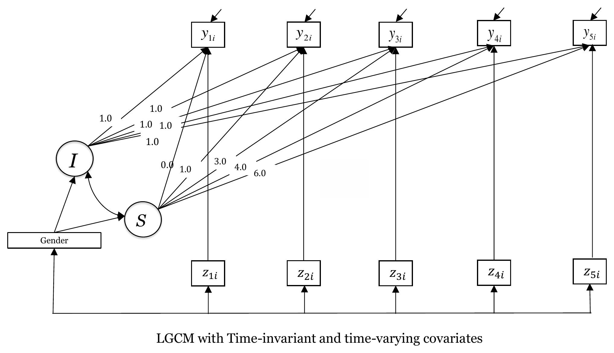 ![Path diagram of the latent growth model with a time-invariant covariate (`female`) and time-varying covariates (hostility at each wave). Look at the arrows from each $z$ to the $y$ of the same wave, and at the two arrows from the gender box to $I$ and $S$. Source: workshop slides [@anyan2023workshop].](../images/slides/slide_51.png){#fig-combined-diagram fig-alt="Path diagram of a linear growth model with intercept and slope factors, five time-varying covariates z1 to z5 pointing to outcomes y1 to y5, and a gender covariate pointing to the intercept and the slope" width="90%"} ## The formal model For participant $i$ at wave $t$, with time scores $\lambda_t = 0, 1, 3, 4, 6$ and hostility $z_{ti}$, $$ y_{ti} = \eta_{0i} + \lambda_t \eta_{1i} + \beta_t z_{ti} + \epsilon_{ti} $$ $$ \eta_{0i} = \alpha_0 + \gamma_0 \,\text{female}_i + \zeta_{0i}, \qquad \eta_{1i} = \alpha_1 + \gamma_1 \,\text{female}_i + \zeta_{1i} $$ In the time-varying covariate model of @sec-tvc the five coefficients $\beta_1, \dots, \beta_5$ were estimated freely. Here they are held equal, $$ \beta_1 = \beta_2 = \beta_3 = \beta_4 = \beta_5 = \beta . $$ The covariances of hostility with the growth factors are fixed at zero, $$ \text{Cov}(\zeta_0, z_t) = 0, \qquad \text{Cov}(\zeta_1, z_t) = 0, \qquad t = 1, \dots, 5 , $$ while the covariances of $\text{female}$ with $z_1, \dots, z_5$ and among $z_1, \dots, z_5$ are estimated freely, together with the means of the covariates. Two things follow from the equations. First, $\eta_{0i}$ is now the initial level of a participant with $\text{female} = 0$ and with a hostility score of zero, and $\alpha_0$ is the mean of that quantity. Second, $\gamma_0$ and $\gamma_1$ describe differences in the growth factors between the two groups after the hostility term has been taken out of the loneliness scores. ## R implementation The syntax below is the one used in the workshop. The model string, the labels and the constraints are not changed. ```{r} #| label: model-combined timeinvartimevar <- ' i =~ 1*lone1 + 1*lone2 + 1*lone3 + 1*lone4 + 1*lone5 s =~ 0*lone1 + 1*lone2 + 3*lone3 + 4*lone4 + 6*lone5 # Time-varying covariates held equal lone1 ~ eq*host1 lone2 ~ eq*host2 lone3 ~ eq*host3 lone4 ~ eq*host4 lone5 ~ eq*host5 # Time invariant covariates i ~ female s ~ female #Estimate the means of TVC and TIC host1 ~ 1 host2 ~ 1 host3 ~ 1 host4 ~ 1 host5 ~ 1 female ~ 1 #Estimate covariances between TIC with TVC female ~~ host1 + host2 + host3 + host4 + host5 host1 ~~ host2 + host3 + host4 + host5 host2 ~~ host3 + host4 + host5 host3 ~~ host4 + host5 host4 ~~ host5 #Fix covariances between TVC and growth factors to zero i ~~ 0*host1 i ~~ 0*host2 i ~~ 0*host3 i ~~ 0*host4 i ~~ 0*host5 s ~~ 0*host1 s ~~ 0*host2 s ~~ 0*host3 s ~~ 0*host4 s ~~ 0*host5 ' fit_timeinvar_timevar <- growth(timeinvartimevar, data = data) summary(fit_timeinvar_timevar, fit.measures = TRUE) ``` Read the syntax in blocks. The five lines `lone1 ~ eq*host1` to `lone5 ~ eq*host5` look like the ones in @sec-tvc, but every coefficient carries the same label `eq`. In lavaan, parameters that share a label are estimated as one value, so the five paths are held equal. The two lines `i ~ female` and `s ~ female` come from @sec-tic. The lines with `~ 1` ask for the means of the covariates, and the `~~` lines estimate the covariances among the covariates. The last two blocks use the `0*` device, which we used earlier to fix loadings, now to fix covariances at zero. ```{r} #| label: extract-main #| include: false pf <- function(p) ifelse(p < .001, "< .001", sub("^0", "", formatC(p, format = "f", digits = 3))) pe <- parameterEstimates(fit_timeinvar_timevar) fm <- fitMeasures(fit_timeinvar_timevar) getp <- function(pe, lhs, op, rhs, col = "est") pe[pe$lhs == lhs & pe$op == op & pe$rhs == rhs, col][1] b_eq <- getp(pe, "lone1", "~", "host1") b_se <- getp(pe, "lone1", "~", "host1", "se") b_z <- getp(pe, "lone1", "~", "host1", "z") g0 <- getp(pe, "i", "~", "female"); g0_se <- getp(pe, "i", "~", "female", "se") g0_z <- getp(pe, "i", "~", "female", "z") g1 <- getp(pe, "s", "~", "female"); g1_se <- getp(pe, "s", "~", "female", "se") g1_p <- getp(pe, "s", "~", "female", "pvalue") g1_lo <- getp(pe, "s", "~", "female", "ci.lower"); g1_hi <- getp(pe, "s", "~", "female", "ci.upper") a0 <- getp(pe, "i", "~1", ""); a0_se <- getp(pe, "i", "~1", "", "se") a1 <- getp(pe, "s", "~1", ""); a1_se <- getp(pe, "s", "~1", "", "se"); a1_p <- getp(pe, "s", "~1", "", "pvalue") v_i <- getp(pe, "i", "~~", "i"); v_s <- getp(pe, "s", "~~", "s"); c_is <- getp(pe, "i", "~~", "s") c_is_se <- getp(pe, "i", "~~", "s", "se") m_fem <- getp(pe, "female", "~1", "") # covariances female with hostility, and correlations fh <- pe[pe$op == "~~" & pe$lhs %in% paste0("host", 1:5) & pe$rhs == "female", ] vf <- getp(pe, "female", "~~", "female") vh <- sapply(paste0("host", 1:5), function(h) getp(pe, h, "~~", h)) r_fh <- fh$est / sqrt(vf * vh[fh$lhs]) # covariances among hostility scores hh <- pe[pe$op == "~~" & pe$lhs %in% paste0("host", 1:4) & grepl("^host", pe$rhs) & pe$lhs != pe$rhs, ] # implied mean of lone1 imp1 <- fitted(fit_timeinvar_timevar)$mean[["lone1"]] m_host1 <- getp(pe, "host1", "~1", "") n_used <- lavInspect(fit_timeinvar_timevar, "nobs") cc_lh <- complete.cases(data[c(paste0("lone", 1:5), paste0("host", 1:5))]) n_extra <- sum(cc_lh & is.na(data$female)) ``` ```{r} #| label: compare-models #| include: false timevaryingcov <- ' i =~ 1*lone1 + 1*lone2 + 1*lone3 + 1*lone4 + 1*lone5 s =~ 0*lone1 + 1*lone2 + 3*lone3 + 4*lone4 + 6*lone5 lone1 ~ host1 lone2 ~ host2 lone3 ~ host3 lone4 ~ host4 lone5 ~ host5 host1 ~ 1 host2 ~ 1 host3 ~ 1 host4 ~ 1 host5 ~ 1 host1 ~~ host2 + host3 + host4 + host5 host2 ~~ host3 + host4 + host5 host3 ~~ host4 + host5 host4 ~~ host5' fit_tvc <- growth(timevaryingcov, data = data) timeinvar <- ' i =~ 1*lone1 + 1*lone2 + 1*lone3 + 1*lone4 + 1*lone5 s =~ 0*lone1 + 1*lone2 + 3*lone3 + 4*lone4 + 6*lone5 i ~ female s ~ female' fit_tic <- growth(timeinvar, data = data) pe5 <- parameterEstimates(fit_tvc); pe6 <- parameterEstimates(fit_tic) fm5 <- fitMeasures(fit_tvc); fm6 <- fitMeasures(fit_tic) b5 <- pe5[pe5$op == "~" & pe5$lhs %in% paste0("lone", 1:5), "est"] cmp <- data.frame( Quantity = c("N used", "Hostility effect", "Female on intercept (SE)", "Female on slope (SE)", "Mean of intercept", "Mean of slope (SE)", "Variance of intercept", "Variance of slope", "Covariance intercept, slope", "CFI", "RMSEA"), `Time-varying only` = c(lavInspect(fit_tvc, "nobs"), paste0(f3(min(b5)), " to ", f3(max(b5))), "", "", f3(getp(pe5, "i", "~1", "")), paste0(f3(getp(pe5, "s", "~1", "")), " (", f3(getp(pe5, "s", "~1", "", "se")), ")"), f3(getp(pe5, "i", "~~", "i")), f4(getp(pe5, "s", "~~", "s")), f4(getp(pe5, "i", "~~", "s")), f3(fm5[["cfi"]]), f3(fm5[["rmsea"]])), `Time-invariant only` = c(lavInspect(fit_tic, "nobs"), "", paste0(f3(getp(pe6, "i", "~", "female")), " (", f3(getp(pe6, "i", "~", "female", "se")), ")"), paste0(f3(getp(pe6, "s", "~", "female")), " (", f3(getp(pe6, "s", "~", "female", "se")), ")"), f3(getp(pe6, "i", "~1", "")), paste0(f3(getp(pe6, "s", "~1", "")), " (", f3(getp(pe6, "s", "~1", "", "se")), ")"), f3(getp(pe6, "i", "~~", "i")), f4(getp(pe6, "s", "~~", "s")), f4(getp(pe6, "i", "~~", "s")), f3(fm6[["cfi"]]), f3(fm6[["rmsea"]])), Combined = c(lavInspect(fit_timeinvar_timevar, "nobs"), f3(b_eq), paste0(f3(g0), " (", f3(g0_se), ")"), paste0(f3(g1), " (", f3(g1_se), ")"), f3(a0), paste0(f3(a1), " (", f3(a1_se), ")"), f3(v_i), f4(v_s), f4(c_is), f3(fm[["cfi"]]), f3(fm[["rmsea"]])), check.names = FALSE ) g0_6 <- getp(pe6, "i", "~", "female"); g0_6_se <- getp(pe6, "i", "~", "female", "se") g1_6 <- getp(pe6, "s", "~", "female") vi5 <- getp(pe5, "i", "~~", "i"); vi6 <- getp(pe6, "i", "~~", "i") a0_5 <- getp(pe5, "i", "~1", "") ``` ## Understanding the output ### Sample, convergence and fit lavaan reports that the estimation ended normally after `r lavInspect(fit_timeinvar_timevar, "iterations")` iterations. The model has `r fm[["npar"]]` free parameters. The output lists `r fm[["npar"]] + 4` parameters and 4 equality constraints, because the five hostility paths count as five parameters until they are held equal. The number of observations used is `r n_used` out of the 442 rows, because the workshop fit uses listwise deletion (see @sec-prelims). Of the 27 rows with a missing value on `female`, only `r n_extra` was not already dropped because of missing loneliness or hostility scores. Remember to report this N when you present the model. Lavaan gives no warning for this model. The latent covariance matrix of the intercept and slope factors is positive definite. The slope factor has very little variance, with a residual variance of `r f4(v_s)`, and the smallest eigenvalue of the latent covariance matrix is `r f4(min(eigen(lavInspect(fit_timeinvar_timevar, "cov.lv"), only.values = TRUE)$values))`. Both are small, so the model sits close to the boundary where a warning would appear, but both are positive. The global fit is as follows. ```{r} #| label: fit-table #| echo: false fit_tab <- data.frame( Index = c(paste0("Chi-square (df = ", fm[["df"]], ")"), "CFI", "TLI", "RMSEA [90% CI]", "SRMR"), Value = c(f3(fm[["chisq"]]), f3(fm[["cfi"]]), f3(fm[["tli"]]), paste0(f3(fm[["rmsea"]]), " [", f3(fm[["rmsea.ci.lower"]]), ", ", f3(fm[["rmsea.ci.upper"]]), "]"), f3(fm[["srmr"]])) ) knitr::kable(fit_tab, caption = paste0("Global fit of the combined covariates model (listwise deletion, N = ", n_used, ").")) ``` The chi-square test is significant, $p$ `r pf(fm[["pvalue"]])`, so the model is rejected as an exact description of the covariance and mean structure. The CFI of `r f3(fm[["cfi"]])` and the TLI of `r f3(fm[["tli"]])` are above the .95 that is often used as a guide, and the SRMR of `r f3(fm[["srmr"]])` is below .08 [@hu1999cutoff]. The RMSEA is `r f3(fm[["rmsea"]])`, and its 90% confidence interval runs from `r f3(fm[["rmsea.ci.lower"]])` to `r f3(fm[["rmsea.ci.upper"]])`. The point estimate sits between .05 and .08, and the upper limit is above .08. The test of close fit (RMSEA at most .05) is rejected, $p$ = `r pf(fm[["rmsea.pvalue"]])`, and the test that the RMSEA is at least .08 is not rejected, $p$ = `r pf(fm[["rmsea.notclose.pvalue"]])`. Thus the fit is acceptable by the CFI, TLI and SRMR and borderline by the RMSEA. We would describe it as adequate and not as a close fit. The baseline chi-square is `r f3(fm[["baseline.chisq"]])` on `r fm[["baseline.df"]]` degrees of freedom, which is very large because many observed variables are strongly correlated, among them loneliness and hostility at the same wave. A large baseline chi-square makes it easier for the CFI to be high, as in @sec-tvc. Loneliness is skewed to the right at all five waves, with skewness between `r f3(min(lone_skew))` and `r f3(max(lone_skew))`, and so is hostility, with skewness between `r f3(min(host_skew))` and `r f3(max(host_skew))`. The maximum likelihood chi-square can be inflated with non-normal data [@curran1996robustness], so the chi-square and the exact value of the RMSEA should be read with the caution given in @sec-prelims. The fit indices of this chapter cannot be compared by a likelihood ratio test with the models of @sec-tvc and @sec-tic. The time-varying covariate model has no `female`, and the time-invariant covariate model has no hostility, so the models contain different observed variables and are not nested. Their chi-square values, AIC [@akaike1974new] and BIC [@schwarz1978estimating] are computed for different sets of variables and for slightly different samples, so they are not on the same scale. ### The estimates The single common coefficient is `r f3(b_eq)` ($SE$ = `r f3(b_se)`, $z$ = `r formatC(b_z, format = "f", digits = 2)`). In the output it appears five times, once for each wave, with the same value and the same standard error, because the five paths are one parameter. A participant with a hostility score one unit higher at a given wave has a loneliness score that is expected to be `r f3(b_eq)` units higher at that wave, given the position on the growth trajectory. The coefficient on the intercept factor is `r f3(g0)` ($SE$ = `r f3(g0_se)`, $z$ = `r formatC(g0_z, format = "f", digits = 2)`), and the coefficient on the slope factor is `r f3(g1)` ($SE$ = `r f3(g1_se)`, $p$ = `r pf(g1_p)`). Participants coded 1 are estimated to have a lower initial level. The difference in the rate of change is small and its 95% confidence interval, from `r f3(g1_lo)` to `r f3(g1_hi)`, includes zero. The covariances of `female` with the five hostility scores run from `r f3(min(fh$est))` to `r f3(max(fh$est))`, and none is distinguishable from zero (the smallest $p$ is `r f3(min(fh$pvalue))`, at wave 2). Expressed as correlations, they run from `r f3(min(r_fh))` to `r f3(max(r_fh))`. Hostility at one wave is clearly related to hostility at the other waves, with covariances from `r f3(min(hh$est))` to `r f3(max(hh$est))`, and the covariances are larger for waves that are close in time. The `i ~~ host` and `s ~~ host` lines in the output show 0.000 without a standard error. Those are the restrictions we fixed, and they are not estimates. The remaining parameters are the means and the variances of the growth factors. The mean of the intercept factor is `r f3(a0)` ($SE$ = `r f3(a0_se)`) and the mean of the slope factor is `r f3(a1)` ($SE$ = `r f3(a1_se)`, $p$ = `r pf(a1_p)`). The residual variances are `r f3(v_i)` for the intercept factor and `r f4(v_s)` for the slope factor, and the residual covariance between them is `r f3(c_is)` ($SE$ = `r f3(c_is_se)`). The variances are residual variances, because the growth factors are now regressed on `female`. The slide in @fig-combined-slide reports the same model. The estimates on the slide were obtained with Mplus. The numbers in this chapter are the ones from the R output above. They agree with the slide for the estimates, the chi-square, the degrees of freedom and the RMSEA. The CFI and TLI on the slide are .973 and .971, whereas lavaan gives `r f3(fm[["cfi"]])` and `r f3(fm[["tli"]])`, and we use the lavaan values. The range of the hostility covariances on the slide (0.037 to 0.161) matches the range in the output, `r f3(min(hh$est))` to `r f3(max(hh$est))`.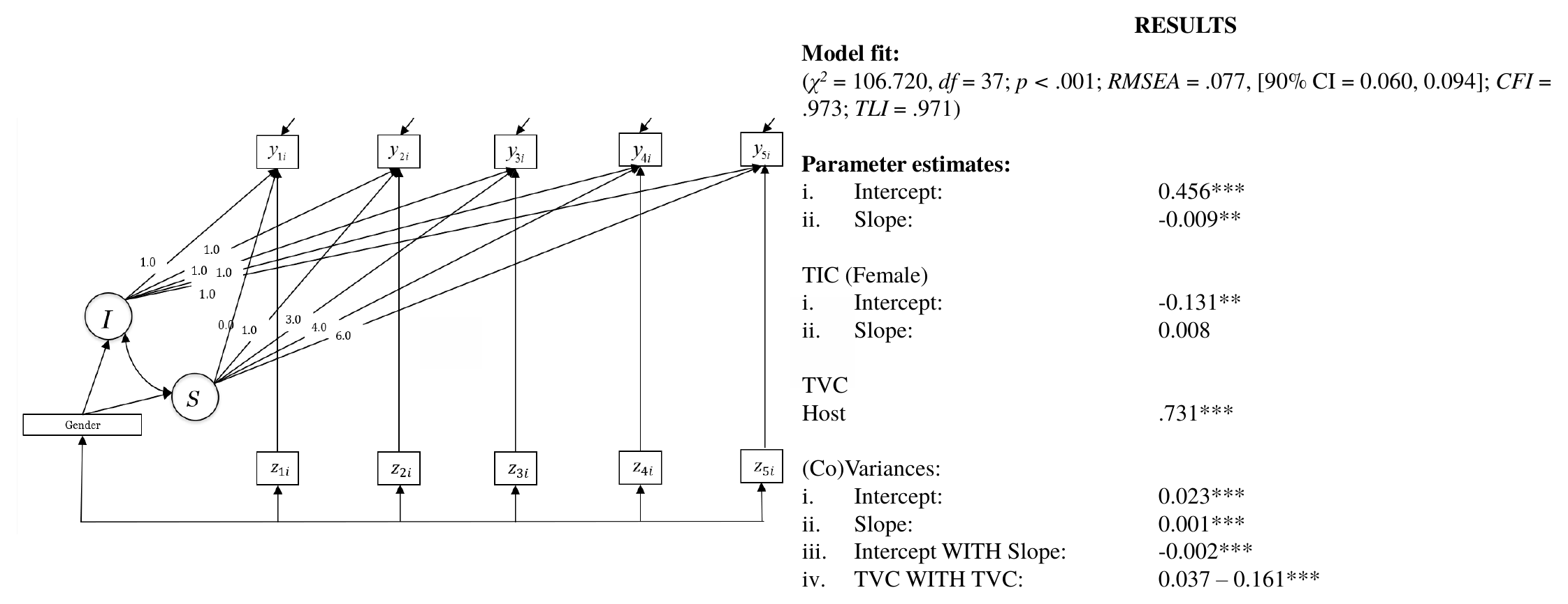 ![Results of the combined model as reported in the workshop. The right-hand panel lists the fit, the growth factor means, the effect of `female` on the growth factors, the common hostility effect and the (co)variances. Look at the value of 0.731 for hostility and at the two `female` coefficients. The slide shows Mplus estimates, and the chapter uses the lavaan output. Source: workshop slides [@anyan2023workshop].](../images/slides/slide_54.png){#fig-combined-slide fig-alt="Path diagram on the left and a results panel on the right with model fit, intercept 0.456, slope -0.009, female effects -0.131 and 0.008, hostility effect 0.731 and variances" width="95%"} ## What the equality constraint means The model of @sec-tvc estimated one hostility coefficient per wave. They ranged from `r f3(min(b5))` to `r f3(max(b5))`. Here they are replaced by one value. This is a restriction that adds four degrees of freedom to the model, and it says that a one-unit difference in hostility is associated with the same difference in loneliness at every wave. It does not say that hostility has the same level at every wave. The hostility means differ over time, as the output shows (from `r f3(min(pe[pe$op == "~1" & grepl("^host", pe$lhs), "est"]))` to `r f3(max(pe[pe$op == "~1" & grepl("^host", pe$lhs), "est"]))`). The common coefficient `r f3(b_eq)` is a summary of five coefficients that were close to each other in @sec-tvc. The restriction can also be tested directly. This check is an addition to the workshop. We fit the same model with the labels `eq` removed and compare the two models, which are nested, with a chi-square difference test [@bentler1980significance]. ```{r} #| label: check-eq # ADDITION (not part of the workshop): is the equality constraint tenable? timeinvartimevar_free <- gsub("eq\\*", "", timeinvartimevar) fit_free_beta <- growth(timeinvartimevar_free, data = data) lrt_eq <- anova(fit_timeinvar_timevar, fit_free_beta) lrt_eq ``` ```{r} #| label: extract-eq #| include: false pe_fb <- parameterEstimates(fit_free_beta) fb <- pe_fb[pe_fb$op == "~" & pe_fb$rhs %in% paste0("host", 1:5), ] ``` The chi-square difference is `r f3(lrt_eq[2, "Chisq diff"])` on `r lrt_eq[2, "Df diff"]` degrees of freedom, $p$ = `r pf(lrt_eq[2, "Pr(>Chisq)"])`. The reduced model, with one common coefficient, is not rejected. The data do not give a reason to prefer five separate coefficients, which range from `r f3(min(fb$est))` to `r f3(max(fb$est))` in this larger model. Note that a non-significant test does not prove that the effects are equal. It means that this sample cannot distinguish them, and that the simpler model is a reasonable summary. The constraint also changes the mean of the slope factor. In the free version, the mean of the slope factor is `r f3(getp(pe_fb, "s", "~1", ""))` with a standard error of `r f3(getp(pe_fb, "s", "~1", "", "se"))` ($p$ = `r pf(getp(pe_fb, "s", "~1", "", "pvalue"))`). In the constrained model, the standard error is `r f3(a1_se)` and $p$ = `r pf(a1_p)`. The mean slope is estimated more precisely when the hostility coefficients are held equal, so the conclusion about the average rate of change depends on the constraint and should be reported together with it. ## What the zero covariances mean ```{r} #| label: check-default # ADDITION (not part of the workshop): leave out the lines that fix the covariances at zero timeinvartimevar_nozero <- sub("#Fix covariances between TVC and growth factors to zero.*$", "", timeinvartimevar) fit_nozero <- growth(timeinvartimevar_nozero, data = data) same_fit <- c(fitMeasures(fit_nozero, "chisq"), fitMeasures(fit_nozero, "npar")) ``` The 10 covariances between the hostility scores and the growth factors are fixed at zero. The reason given in the workshop is to keep the model simple and to help it converge, because every extra covariance is an extra parameter. It is also the case that lavaan treats exogenous observed covariates this way by default, so the lines make explicit what the program would otherwise do silently. Leaving the 10 lines out gives the same chi-square (`r f3(same_fit[["chisq"]])` against `r f3(fm[["chisq"]])`) and the same number of free parameters (`r same_fit[["npar"]]` against `r fm[["npar"]]`). The substantive meaning is more important. Fixing $\text{Cov}(\zeta_0, z_t) = 0$ says that, after the effect of `female` is removed, a participant's initial level and rate of change are unrelated to the hostility scores of that participant. All of the association between hostility and loneliness is assigned to the wave-specific regression with coefficient $\beta$. This is a strong assumption. If participants who are more hostile on average are also lonelier on average, beyond what the same-wave regression captures, then that stable part of the association has nowhere to go in the model except into $\beta$. The coefficient $\beta$ then mixes a within-person association with a between-person one. Separating the two requires modeling choices that go beyond this chapter [@curran2011disaggregation]. The check below is again an addition to the workshop. It frees the 10 covariances. The model converges without difficulty in this dataset. ```{r} #| label: check-cov # ADDITION (not part of the workshop): free the covariances of the TVC with the growth factors timeinvartimevar_cov <- paste( sub("#Fix covariances between TVC and growth factors to zero.*$", "", timeinvartimevar), "i ~~ host1 + host2 + host3 + host4 + host5 s ~~ host1 + host2 + host3 + host4 + host5") fit_cov <- growth(timeinvartimevar_cov, data = data) lrt_cov <- anova(fit_timeinvar_timevar, fit_cov) lrt_cov ``` ```{r} #| label: extract-cov #| include: false pe_c <- parameterEstimates(fit_cov) fmc <- fitMeasures(fit_cov) ci <- pe_c[pe_c$op == "~~" & pe_c$lhs == "i" & grepl("^host", pe_c$rhs), ] si <- pe_c[pe_c$op == "~~" & pe_c$lhs == "s" & grepl("^host", pe_c$rhs), ] ``` The restricted model is rejected, with a chi-square difference of `r f3(lrt_cov[2, "Chisq diff"])` on `r lrt_cov[2, "Df diff"]` degrees of freedom ($p$ `r pf(lrt_cov[2, "Pr(>Chisq)"])`). The fit of the model with free covariances is better (CFI `r f3(fmc[["cfi"]])`, RMSEA `r f3(fmc[["rmsea"]])`). The covariances of the intercept factor with hostility are positive, from `r f3(min(ci$est))` to `r f3(max(ci$est))`, and `r sum(ci$pvalue < .01)` of the `r nrow(ci)` have $p$ < .01. Those of the slope factor are close to zero and mostly small, from `r f3(min(si$est))` to `r f3(max(si$est))`. The pattern suggests that participants with a higher initial level of loneliness, after the same-wave hostility term has been taken out, also tend to have higher hostility scores at waves 2 to 5. With the covariances free, the common hostility coefficient is `r f3(getp(pe_c, "lone1", "~", "host1"))` instead of `r f3(b_eq)`, the `female` coefficient on the intercept is `r f3(getp(pe_c, "i", "~", "female"))` and the one on the slope is `r f3(getp(pe_c, "s", "~", "female"))`. The conclusions about `female` do not change, and the hostility coefficient is a little smaller. We therefore keep the workshop model as the one to interpret, and we read the hostility coefficient as the association between hostility and loneliness at the same wave under the assumption that the growth factors are unrelated to hostility. ## Sensitivity to the missing data handling The workshop model uses listwise deletion, and `r n_used` of the 442 rows are used. Listwise deletion, FIML and the missing at random assumption are explained in @sec-prelims. In the conditions examined in one simulation study, FIML performed better than listwise deletion [@enders2001relative]. The check below is an addition to the workshop. The same model syntax is fitted with `missing = "fiml"` and `fixed.x = FALSE`. The second argument is needed because lavaan otherwise treats `female` and the hostility scores as fixed and cannot use a row where one of them is missing. With `fixed.x = FALSE`, the means, variances and covariances of the covariates are estimated. ```{r} #| label: fiml-extract #| include: false est_diag <- read.csv("data/diag/estimates_listwise_vs_fiml.csv") sum_diag <- read.csv("data/diag/diagnostics_summary.csv") e7 <- est_diag[est_diag$label == "007_timeinvar_timevar", ] s7 <- sum_diag[sum_diag$label == "007_timeinvar_timevar", ] gete <- function(lhs, op, rhs) e7[e7$lhs == lhs & e7$op == op & e7$rhs == rhs, ][1, ] rows <- list( "Hostility effect (eq)" = gete("lone1", "~", "host1"), "Female on intercept" = gete("i", "~", "female"), "Female on slope" = gete("s", "~", "female"), "Mean of intercept" = gete("i", "~1", ""), "Mean of slope" = gete("s", "~1", ""), "Residual variance of intercept" = gete("i", "~~", "i"), "Residual variance of slope" = gete("s", "~~", "s"), "Covariance intercept, slope" = gete("i", "~~", "s") ) fiml_tab <- data.frame( Parameter = names(rows), Listwise = sapply(rows, function(r) f4(r$est_lw)), `SE listwise` = sapply(rows, function(r) f4(r$se_lw)), FIML = sapply(rows, function(r) f4(r$est_fiml)), `SE FIML` = sapply(rows, function(r) f4(r$se_fiml)), check.names = FALSE, row.names = NULL ) z_slope_fiml <- rows[["Female on slope"]]$est_fiml / rows[["Female on slope"]]$se_fiml ``` ```{r} #| label: tbl-fiml #| echo: false #| tbl-cap: "Estimates of the combined model under listwise deletion (workshop) and under FIML with fixed.x = FALSE." knitr::kable(fiml_tab) ``` The FIML analysis uses `r s7$n_fiml` rows. In @tbl-fiml, the point estimates are close to the listwise ones for the hostility effect, the mean of the intercept and the mean of the slope. The `female` coefficient on the intercept is somewhat larger in absolute value under FIML (`r f3(rows[["Female on intercept"]]$est_fiml)` against `r f3(rows[["Female on intercept"]]$est_lw)`), and both residual variances are larger (for the intercept factor, `r f4(rows[["Residual variance of intercept"]]$est_fiml)` against `r f4(rows[["Residual variance of intercept"]]$est_lw)`, and for the slope factor, `r f4(rows[["Residual variance of slope"]]$est_fiml)` against `r f4(rows[["Residual variance of slope"]]$est_lw)`). The one result that changes in kind is the `female` coefficient on the slope. Under FIML it is `r f3(rows[["Female on slope"]]$est_fiml)` with a standard error of `r f3(rows[["Female on slope"]]$se_fiml)`, which gives $z$ = `r formatC(z_slope_fiml, format = "f", digits = 2)`, while under listwise deletion it is `r f3(g1)` with $p$ = `r pf(g1_p)`. The estimates are similar, but the inference is not. Thus we would not claim that the difference in the rate of change by `female` is absent, and we would not claim that it is established either. The data are consistent with a small difference, and the answer depends on how the missing data are handled. The fit under FIML is similar to the listwise fit: the chi-square is `r f3(s7$chisq_fiml)`, the CFI is `r f3(s7$cfi_fiml)`, the RMSEA is `r f3(s7$rmsea_fiml)` and the SRMR is `r f3(s7$srmr_fiml)`. With the MLR estimator, which corrects the test statistic and the standard errors for non-normality [@yuan2000three], the robust CFI is `r f3(s7$cfi_mlr)` and the robust RMSEA is `r f3(s7$rmsea_mlr)`, with a scaled chi-square of `r f3(s7$chisq_mlr_scaled)`. The scaled chi-square is smaller than the ML chi-square under FIML (`r f3(s7$chisq_fiml)`). The conclusions about fit do not change. ## Interpretation Across the five waves, a difference of one unit in hostility is associated with a difference of `r f3(b_eq)` units in loneliness at the same wave, given the growth trajectory and `female`. The standard error is small, `r f3(b_se)`, and holding the coefficient equal across waves does not worsen the fit in a way the data can detect. It is an association, and the model does not tell us whether hostility affects loneliness, the other way around, or neither. Because the zero covariances are an assumption, the value is the same-wave association under that assumption. Participants coded 1 on `female` are estimated to have a lower initial level than participants coded 0, at the same level of hostility (`r f3(g0)`). The estimated difference in the yearly rate of change is small (`r f3(g1)`), and over the six years from the first to the last wave it adds up to `r f3(6 * g1)` units. The interval for the slope coefficient includes zero under listwise deletion and the FIML result leans the other way, so we describe the evidence for a group difference in the rate of change as weak and sensitive to the missing data handling. The intercept mean of `r f3(a0)` is the expected loneliness at the first wave for a participant coded 0 on `female` with a hostility score of zero. Zero is outside the observed range of hostility (`r host_range[1]` to `r host_range[2]`), so the number is an extrapolation and not the typical starting level. It should not be compared with the intercepts of the earlier chapters. Centering hostility is shown in @sec-tvc. In the range of the data, the model-implied mean of loneliness at the first wave is `r f3(imp1)`, computed at the mean hostility of the first wave (`r f3(m_host1)`) and the average of `female` (`r f3(m_fem)`). The mean of the slope factor is `r f3(a1)` per year for participants coded 0 on `female`. The evidence for a nonzero mean slope is stronger here than in the version with free hostility coefficients ($p$ = `r pf(a1_p)` against $p$ = `r pf(getp(pe_fb, "s", "~1", "", "pvalue"))`), for the reason given in the section on the equality constraint. ## What changed compared with the previous models @tbl-compare puts the three models side by side. The numbers for the models of @sec-tvc and @sec-tic come from fits with their workshop syntax. ```{r} #| label: tbl-compare #| echo: false #| tbl-cap: "Selected estimates from the time-varying covariate model, the time-invariant covariate model and the combined model (listwise deletion in all three). The variances are residual variances of the growth factors." knitr::kable(cmp) ``` Compared with the time-invariant covariate model, the `female` coefficient on the intercept factor is `r f3(g0)` here and `r f3(g0_6)` there, so it has not moved. The coefficient on the slope factor is `r f3(g1)` here and `r f3(g1_6)` there. What changed is the precision. The standard error of the intercept coefficient fell from `r f3(g0_6_se)` to `r f3(g0_se)`, and the residual variance of the intercept factor fell from `r f3(vi6)` to `r f3(v_i)`. Most of the residual between-person variance of the intercept disappears once hostility is in the model, and a smaller residual variance goes with a more precise estimate of the group difference. A likely reason why the coefficient did not move is that `female` is nearly unrelated to hostility in these data. The covariances between them are small, and the correlations run only from `r f3(min(r_fh))` to `r f3(max(r_fh))`. When two predictors are nearly uncorrelated, adding one of them changes the coefficient of the other very little. Compared with the time-varying covariate model, the single hostility coefficient of `r f3(b_eq)` sits inside the range of the five coefficients of that model, `r f3(min(b5))` to `r f3(max(b5))`. The residual variance of the intercept factor is `r f3(v_i)` against `r f3(vi5)`. This difference is not due to `female` alone, because the combined model also holds the hostility coefficients equal and uses one row fewer (`r n_used` against `r lavInspect(fit_tvc, "nobs")`). The intercept mean is `r f3(a0)` here and `r f3(a0_5)` there. These two numbers are not the same quantity. In the combined model the mean refers to participants coded 0 on `female`. Averaging over the two groups gives `r f3(a0 + g0 * m_fem)`, which is near the value of the time-varying covariate model. The fit indices of the combined model are CFI `r f3(fm[["cfi"]])` and RMSEA `r f3(fm[["rmsea"]])`, against `r f3(fm5[["cfi"]])` and `r f3(fm5[["rmsea"]])` for the time-varying covariate model and `r f3(fm6[["cfi"]])` and `r f3(fm6[["rmsea"]])` for the time-invariant covariate model. The two models with hostility have a high CFI and a borderline RMSEA, as in @sec-tvc. The time-invariant covariate model has a lower CFI and a higher RMSEA. The models contain different observed variables and have different baseline models, so the indices are not used to rank them. ## What this model answers and what it cannot tell The model answers whether the same-wave association of hostility with loneliness and the association of `female` with the growth factors can be estimated together, and whether they change when they are. In these data they do not change much. The hostility coefficient is `r f3(b_eq)` and the `female` coefficient on the intercept is `r f3(g0)`, and both are close to their values in the single-covariate models. The two covariates are close to unrelated in these data. The model cannot tell us why the associations exist or in which direction they act. The zero covariances between hostility and the growth factors are a restriction that the data reject when it is tested, so the hostility coefficient should not be read as a pure within-person effect. The model cannot tell us what the intercept is for a typical participant, because it is defined at a hostility score of zero. It cannot settle the group difference in the rate of change, because the listwise and FIML results lead to different conclusions. It also says nothing about the later outcome that a growth trajectory might predict. That question is taken up in @sec-distal, where the growth factors become predictors instead of outcomes. ## Researcher's perspective Report the N used. The fit used listwise deletion and `r n_used` participants, and the FIML result should be given next to it when it leads to a different conclusion, as it does here for the slope coefficient. Report that the equality constraint was imposed and that the check against the freely estimated version supports it in these data. Report the zero covariances as a restriction. They come from the workshop and from the default of the software. If a reader asks whether hostility is related to the initial level of loneliness beyond the same-wave association, the model as specified cannot answer, and the version with free covariances can. You can run that version as above and report both. ::: {.callout-warning title="Read the intercept with the covariates at zero"} The intercept factor is defined at `female` = 0 and at a hostility score of zero, which is outside the observed range. If the intercept is of substantive interest, center the time-varying covariate as shown in @sec-tvc and refit the model. ::: Remember that only models with acceptable fit should be interpreted substantively. The fit of this model is adequate by the CFI, TLI and SRMR and borderline by the RMSEA, and the scores are skewed (see @sec-prelims). The estimates describe this dataset under these specifications and are not causal effects.