Code
table(data$subs5, useNA = "ifany")
   0    1    2    3    4    5    6    7    8   13 <NA>
193 77 44 31 17 14 2 2 1 1 60 In Chapter 5 the growth factors were the outcomes. A time-invariant covariate was used to explain why participants differ in their initial level and in their rate of change. In this chapter the direction of the arrow is reversed. The intercept factor and the slope factor are used as predictors of a variable that is measured later and only once. Such a variable is called a distal outcome.
The question is whether the way in which loneliness develops over the five waves is related to something measured at the end of the study. Here, the distal outcome is substance use at wave 5 (subs5). A model that only uses the loneliness score at wave 5 as a predictor would ignore where participants started and how fast they moved. Here, the intercept and slope factors stand for the whole trajectory and are both used as predictors.
The linear growth model of Chapter 2 describes every participant by an initial level (the intercept factor i) and a rate of change (the slope factor s). Both factors are latent variables, so their values are never observed directly. They are estimated from the five loneliness scores.
In the distal outcome model, one observed variable is added and regressed on i and s. The regression coefficient of i tells us how much higher or lower the outcome is expected to be for participants whose initial level of loneliness is one unit higher, given the same rate of change. The coefficient of s tells us the same for the rate of change, given the same initial level. Thus, the two coefficients are partial effects, as in any multiple regression.
The advantage over a regression on observed scores is that i and s are free of the wave-specific residuals of the loneliness scores.
The dataset has five waves of loneliness (lone1 to lone5) and one measurement of substance use at wave 5 (subs5). We use the time scores 0, 1, 3, 4 and 6 as before, so the intercept refers to the first wave (2015) and the slope is the change per year.
Before fitting the model, we look at the outcome.
table(data$subs5, useNA = "ifany")
0 1 2 3 4 5 6 7 8 13 <NA>
193 77 44 31 17 14 2 2 1 1 60 The variable takes the values 0 to 13 and is observed for 382 of the 442 participants. Of these, 193 have a score of zero, and only 4 have a score above 6. The distribution is therefore strongly right skewed (skewness 2.14, excess kurtosis 7.53). Note that the model treats the outcome as continuous and normal.
The measurement part is the linear growth model. For participant \(i\) at wave \(t\),
\[ y_{ti} = \eta_{0i} + \lambda_t \, \eta_{1i} + \varepsilon_{ti}, \]
where \(\eta_{0i}\) is the intercept factor, \(\eta_{1i}\) is the slope factor, and the time scores are \(\lambda_t = 0, 1, 3, 4, 6\). The growth factors vary around their means,
\[ \eta_{0i} = \alpha_0 + \zeta_{0i}, \qquad \eta_{1i} = \alpha_1 + \zeta_{1i}, \]
and the two factors are allowed to covary. The distal outcome \(z_i\) (here subs5) is added as a regression on both factors,
\[ z_i = \alpha_z + \gamma_0 \, \eta_{0i} + \gamma_1 \, \eta_{1i} + \zeta_{zi}. \]
The parameter \(\gamma_0\) is the effect of the initial level and \(\gamma_1\) is the effect of the rate of change. The term \(\alpha_z\) is the expected outcome when both growth factors are zero, and the variance of \(\zeta_{zi}\) is the part of the outcome not accounted for by the growth factors. No covariance between \(\zeta_{zi}\) and the residuals \(\varepsilon_{ti}\) is estimated in this specification. The diagram in Figure 7.1 shows the model as it was presented in the workshop.
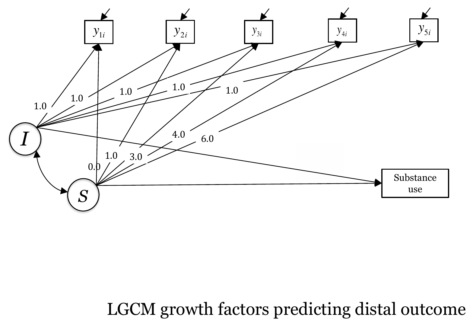
The model uses the same growth specification as the linear growth model in Chapter 2. The only addition is the regression subs5 ~ i + s. The line subs5 ~ 1 frees the intercept of subs5. Without it, lavaan fixes this intercept to zero, which adds a restriction to the model.
distal <- ' i =~ 1*lone1 + 1*lone2 + 1*lone3 + 1*lone4 + 1*lone5
            s =~ 0*lone1 + 1*lone2 + 3*lone3 + 4*lone4 + 6*lone5

# Time invariant covariates
subs5 ~ i + s

#Estimate the intercept of subs
subs5 ~ 1'
fit_distal <- growth(distal, data = data)
summary(fit_distal, fit.measures = TRUE)
lavaan 0.6.17 ended normally after 62 iterations
Estimator ML
Optimization method NLMINB
Number of model parameters 14
Used Total
Number of observations 290 442
Model Test User Model:
Test statistic 74.672
Degrees of freedom 13
P-value (Chi-square) 0.000
Model Test Baseline Model:
Test statistic 438.031
Degrees of freedom 15
P-value 0.000
User Model versus Baseline Model:
Comparative Fit Index (CFI) 0.854
Tucker-Lewis Index (TLI) 0.832
Loglikelihood and Information Criteria:
Loglikelihood user model (H0) -1240.424
Loglikelihood unrestricted model (H1) -1203.087
Akaike (AIC) 2508.847
Bayesian (BIC) 2560.226
Sample-size adjusted Bayesian (SABIC) 2515.829
Root Mean Square Error of Approximation:
RMSEA 0.128
90 Percent confidence interval - lower 0.101
90 Percent confidence interval - upper 0.157
P-value H_0: RMSEA <= 0.050 0.000
P-value H_0: RMSEA >= 0.080 0.998
Standardized Root Mean Square Residual:
SRMR 0.086
Parameter Estimates:
Standard errors Standard
Information Expected
Information saturated (h1) model Structured
Latent Variables:
Estimate Std.Err z-value P(>|z|)
i =~
lone1 1.000
lone2 1.000
lone3 1.000
lone4 1.000
lone5 1.000
s =~
lone1 0.000
lone2 1.000
lone3 3.000
lone4 4.000
lone5 6.000
Regressions:
Estimate Std.Err z-value P(>|z|)
subs5 ~
i 0.896 0.398 2.251 0.024
s 5.889 3.222 1.828 0.068
Covariances:
Estimate Std.Err z-value P(>|z|)
i ~~
s -0.015 0.003 -5.793 0.000
Intercepts:
Estimate Std.Err z-value P(>|z|)
.subs5 -0.006 0.539 -0.011 0.991
i 1.466 0.025 58.598 0.000
s -0.023 0.004 -5.114 0.000
Variances:
Estimate Std.Err z-value P(>|z|)
.lone1 0.055 0.011 5.231 0.000
.lone2 0.118 0.012 9.727 0.000
.lone3 0.171 0.015 11.052 0.000
.lone4 0.122 0.012 10.569 0.000
.lone5 0.052 0.011 4.929 0.000
.subs5 2.365 0.200 11.825 0.000
i 0.142 0.016 8.925 0.000
s 0.003 0.001 5.308 0.000Notice the first lines of the output. The model uses 290 of the 442 rows. As explained in Chapter 1, the workshop script uses listwise deletion. The loneliness scores are complete for 321 participants, and subs5 is missing for another 31 of these, which leaves 290. In total, 152 rows (34%) do not contribute to this model. This is a larger loss than for the linear growth model alone (321 rows).
The chi-square test of the model is 74.672 on 13 degrees of freedom and is rejected. The fit indices are CFI = .854, TLI = .832, RMSEA = .128 and SRMR = .086. Following the usual combination rules (Hu & Bentler, 1999), these values do not indicate a good fit. The RMSEA is well above the customary limit, and its 90% confidence interval (0.101 to 0.157) does not include values that are conventionally regarded as acceptable. The fit statistics are the same as the ones on the workshop slide in Figure 7.2.
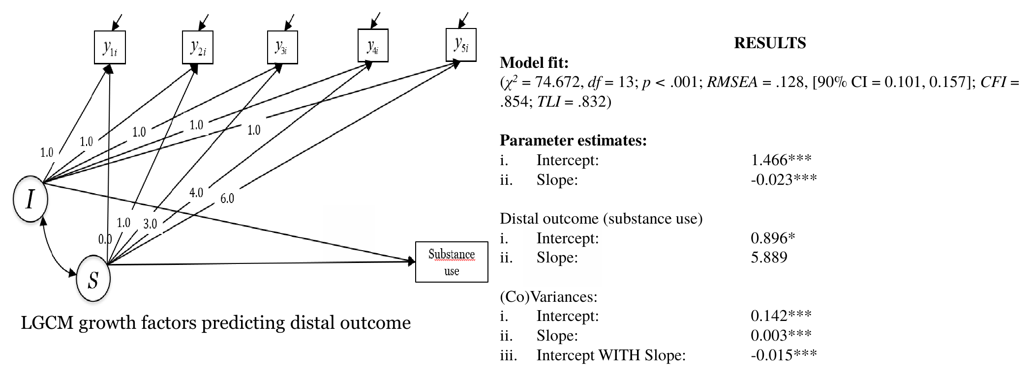
On the slide, “Intercept” and “Slope” under “Distal outcome” are the lines subs5 ~ i and subs5 ~ s in the lavaan output. The intercept of subs5 itself is a different parameter and is not on the slide.
The misfit is mostly inherited from the growth part of the model. We can check this with a short addition that was not part of the workshop. The linear growth model without the distal outcome is fitted to the same 290 participants, and its fit is compared with the fit above.
# Addition, not part of the workshop: linear growth model without subs5,
# fitted to the same participants as the distal outcome model
linear_only <- ' i =~ 1*lone1 + 1*lone2 + 1*lone3 + 1*lone4 + 1*lone5
                 s =~ 0*lone1 + 1*lone2 + 3*lone3 + 4*lone4 + 6*lone5'
fit_lin_same <- growth(linear_only, data = data[cc_all, ])
round(fitMeasures(fit_lin_same, c("chisq", "df", "cfi", "rmsea")), 3)
chisq df cfi rmsea
67.954 10.000 0.861 0.141 The linear model alone has a chi-square of 67.954 on 10 degrees of freedom, CFI = .861 and RMSEA = .141. Adding the outcome and the regression adds 3 degrees of freedom and increases the chi-square by about 6.7. Thus, most of the lack of fit comes from the way in which a straight line describes the five loneliness scores, and little of it comes from the regression on the outcome. Remember that the growth factors come from a model that does not fit well, so the coefficients are tentative.
The regression coefficients are the main result.
reg[, c("lhs", "op", "rhs", "est", "se", "z", "pvalue", "ci.lower", "ci.upper")] lhs op rhs est se z pvalue ci.lower ci.upper
11 subs5 ~ i 0.896 0.398 2.251 0.024 0.116 1.676
12 subs5 ~ s 5.889 3.222 1.828 0.068 -0.426 12.203The other parameters of interest are the means, variances and covariance of the growth factors, which can be read in the summary above. The mean of the intercept factor is 1.466 and the mean of the slope factor is -0.023 per year. The variances are 0.142 for the intercept factor and 0.003 for the slope factor, and the covariance of the two factors is -0.015. These match the values on the slide, and they are close to those of the linear growth model of Chapter 2 (an intercept of 1.466 and a slope of -0.025 with 321 participants).
The coefficient of i is 0.896 (standard error 0.398, p = .024). This means that, holding the rate of change constant, a participant whose initial level of loneliness is one unit higher is expected to have a subs5 score that is about 0.9 units higher. The estimate is statistically different from zero at the .05 level, although the 95% confidence interval is wide (from 0.12 to 1.68).
The coefficient of s is 5.889 (standard error 3.222, p = .068). The estimate is large in absolute size, but the standard error is also large, and the 95% confidence interval runs from -0.43 to 12.20. It includes zero, and the estimate is not statistically different from zero at the .05 level. The data are consistent with a positive association between a steeper increase in loneliness and higher substance use at wave 5, but they do not establish it. The result for the slope also changes with the handling of missing data, as the next section shows.
The slope factor is measured in units of loneliness per year, and its variance is tiny (0.003, which is a standard deviation of 0.056). A difference of one unit in s is therefore far outside the range of values that occur in the data, and the coefficient of 5.889 is large only because it is expressed per unit of a factor that hardly varies. The size of the coefficient alone does not say that the slope is a stronger predictor than the intercept.
To compare the two predictors, we multiply each coefficient by the standard deviation of its factor. This gives the expected difference in subs5 for a participant who is one standard deviation higher on the factor.
# Expected difference in subs5 for a one standard deviation difference in each factor
c(i = gi * sd_lv["i"], s = gs * sd_lv["s"])
i.i s.s
0.3380402 0.3316519 On this scale the two effects are about equal, roughly 0.34 units for the intercept factor and 0.33 units for the slope factor. The standard deviation of subs5 among the 290 participants is 1.56, so each of these differences is about one fifth of a standard deviation of the outcome. The two growth factors are also strongly and negatively correlated (-0.70). Participants who start higher tend to increase less, and this overlap makes it difficult to separate the two coefficients, which is one reason for the large standard error of the slope coefficient.
The model explains only a small part of the variance of the outcome. The R-squared of subs5 is 0.028, which is about 3%. The estimated intercept of subs5 is -0.006. It is the expected outcome for a participant with i and s both equal to zero, which is a combination far from what is observed, and we do not interpret it.
Because only 290 of 442 rows are used, we refit the model with FIML (see Chapter 1). The code below is an addition that was not part of the workshop.
# Addition, not part of the workshop: same model, FIML instead of listwise deletion
fit_distal_fiml <- growth(distal, data = data, missing = "fiml")
fitMeasures(fit_distal_fiml, c("chisq", "df", "cfi", "rmsea", "srmr"))
chisq df cfi rmsea srmr
76.779 13.000 0.888 0.106 0.074 parameterEstimates(fit_distal_fiml) |>
filter(op == "~") |>
select(lhs, op, rhs, est, se, z, pvalue) lhs op rhs est se z pvalue
1 subs5 ~ i 0.833 0.331 2.514 0.012
2 subs5 ~ s 5.865 2.853 2.056 0.040lavaan reports that some cases are empty and ignored. These are rows without any observed value on the variables of the model, and they leave 438 rows in the analysis. The coefficient of i is 0.833 (standard error 0.331) and the coefficient of s is 5.865 (standard error 2.853). The point estimates are close to the listwise ones, and the standard errors are smaller. The slope coefficient now has p = .040 and the coefficient of the intercept factor has p = .012. Thus, whether the slope is statistically different from zero depends on the handling of missing data, and a cautious reading is that the evidence for the slope is weak. The fit improves somewhat (CFI = .888, RMSEA = .106) but is still not good.
FIML was found to perform better than listwise deletion in the conditions examined by Enders & Bandalos (2001). It rests on the missing at random assumption, and subs5 is missing for 60 participants, so a relation between missingness and the unobserved level of substance use cannot be ruled out.
The model is estimated with maximum likelihood, which assumes that the outcome, given the growth factors, is normally distributed. The variable subs5 has a lower bound at zero, about half of the observed values are zero (193 of 382), and the distribution is skewed. The loneliness scores are also skewed, with skewness between 1.52 and 3.05 across the five waves (see Chapter 1). This has two consequences. The ML chi-square tends to be inflated with non-normal data (Curran et al., 1996), so the fit values above may look somewhat worse than they would with a correction. The standard errors also rest on normality, and the predicted values of a linear regression can fall below zero.
A correction is available in lavaan with the estimator "MLR" (Yuan & Bentler, 2000), which gives robust standard errors and a scaled test statistic.
# Addition, not part of the workshop: robust ML with FIML
fit_distal_mlr <- growth(distal, data = data, estimator = "MLR", missing = "fiml")
fitMeasures(fit_distal_mlr, c("chisq.scaled", "df", "cfi.robust", "rmsea.robust"))
chisq.scaled df cfi.robust rmsea.robust
46.605 13.000 0.896 0.112 With the scaled test statistic, the chi-square is 46.605, CFI = .896 and RMSEA = .112, so the fit remains below the usual standards. A different model for the outcome, such as a count model, is not part of the workshop and is not fitted here.
In Chapter 5 the covariate was a predictor of the growth factors, and the arrows pointed from the observed variable to i and s. In this chapter, the arrows point from i and s to an observed variable. In terms of the lavaan syntax, the growth factors move to the right side of a ~ line. The growth specification, the time scores and the interpretation of the means and variances of the factors are unchanged. What does change is the sample (290 rows instead of 321) and the number of estimated parameters (14), because the outcome adds a regression coefficient for each factor, an intercept and a residual variance.
The model answers the question of whether the initial level and the rate of change of loneliness, estimated from five waves, are statistically associated with substance use at wave 5. In this dataset the association with the initial level is statistically different from zero under listwise deletion, and the association with the slope is uncertain and depends on the handling of missing data. The model also has a poor fit.
The outcome subs5 is measured at wave 5, which is also the wave of the last loneliness score lone5. The slope factor is defined by all five waves, so s already contains information from the time at which subs5 is measured. The growth process and the outcome are not separated in time, and the temporal ordering that the word “predict” suggests is not clean. The regression coefficients describe an association, and they do not show that the trajectory of loneliness leads to substance use. The reverse direction, or a shared influence on both variables, is equally compatible with the data.
Several further limits apply. The model assumes a linear trajectory, and the fit shows that a straight line is only a rough description. No covariance between the residual of subs5 and the residual of lone5 is estimated, although both are measured at wave 5, and this restriction could contribute to the misfit. The estimates also come from 290 of 442 participants. Finally, the model says nothing about whether the relation is the same for different groups, which is the topic of Chapter 8.
Four choices matter when a distal outcome is added to a growth model: the timing of the outcome, the number of waves, the scale of the factors, and missing data.
An outcome measured after the last wave of the growth process allows a clearer ordering than one measured at the same wave, and the design of the data collection sets that limit. If the outcome is at wave 5, a growth model of waves 1 to 4 would give a cleaner temporal ordering at the cost of less information on the slope. This alternative is not fitted here.
Report the standardized or one-standard-deviation effects next to the raw coefficients, as we did above, so that the reader can judge size. Report the number of rows used, say that listwise deletion was applied, and show a FIML result as a check. When the conclusion changes between the two, as for the slope coefficient here, say so and avoid a strong claim.
Report the fit as it is. The model has CFI = .854 and RMSEA = .128, and the results should be described as tentative. The standard errors and the tests are less trustworthy than they are for a well-fitting model. Groups are compared in Chapter 8.