The models in the previous chapters describe one growth process for all participants in the dataset. In Chapter 7 we asked what the initial level and the rate of change of loneliness predict. A different question is whether the growth process is the same in two groups. Here, we ask whether the initial level, the rate of change and the between-person variation are equal in the two groups. A multigroup growth model answers this by fitting the same growth model in each group at the same time and by testing which parameters can be held equal across the groups.
A multiple-group approach to growth models is described in Duncan & Duncan (2004). In the workshop, we used the grouping variable female, which has the values 0 and 1 in the dataset. This chapter follows that analysis. We start with a model in which everything is held equal across the groups and then free one block of parameters at a time.
8.2 The idea in plain language
The growth model has a few parameters: the means of the intercept factor and the slope factor, their variances, their covariance and the residual variance. Holding these parameters equal across the groups says that one set of values describes both groups. Freeing them says that each group has its own set.
The models are built in four steps, and every step is nested in the one before it.
M1 holds everything equal: growth factor means, growth factor variances and covariance, and residual variances.
M2 frees the growth factor means.
M3 also frees the growth factor variances and the covariance.
M4 also frees the residual variances, which are still held equal over time within each group.
M1 versus M2 tests whether the groups differ in their average trajectory. M2 versus M3 tests the extent of between-person differences in the trajectories of the groups. M3 versus M4 tests the extent of within-person variability around the individual trajectories. These are the three questions on the workshop slide in Figure 8.3.
8.3 A concrete example
We use the five loneliness scores (lone1 to lone5) and the time scores 0, 1, 3, 4 and 6, as in the earlier chapters. The grouping variable is female. In the dataset, 222 rows are coded 0, 193 rows are coded 1, and 27 rows have a missing value. The workshop slides call the two groups male and female. Here, we refer to them by their codes. The output of lavaan labels the first group as “Group 1 [0]” and the second as “Group 2 [1]”, and the labels m and f in the syntax follow this order. Thus, m belongs to the group coded 0 and f to the group coded 1.
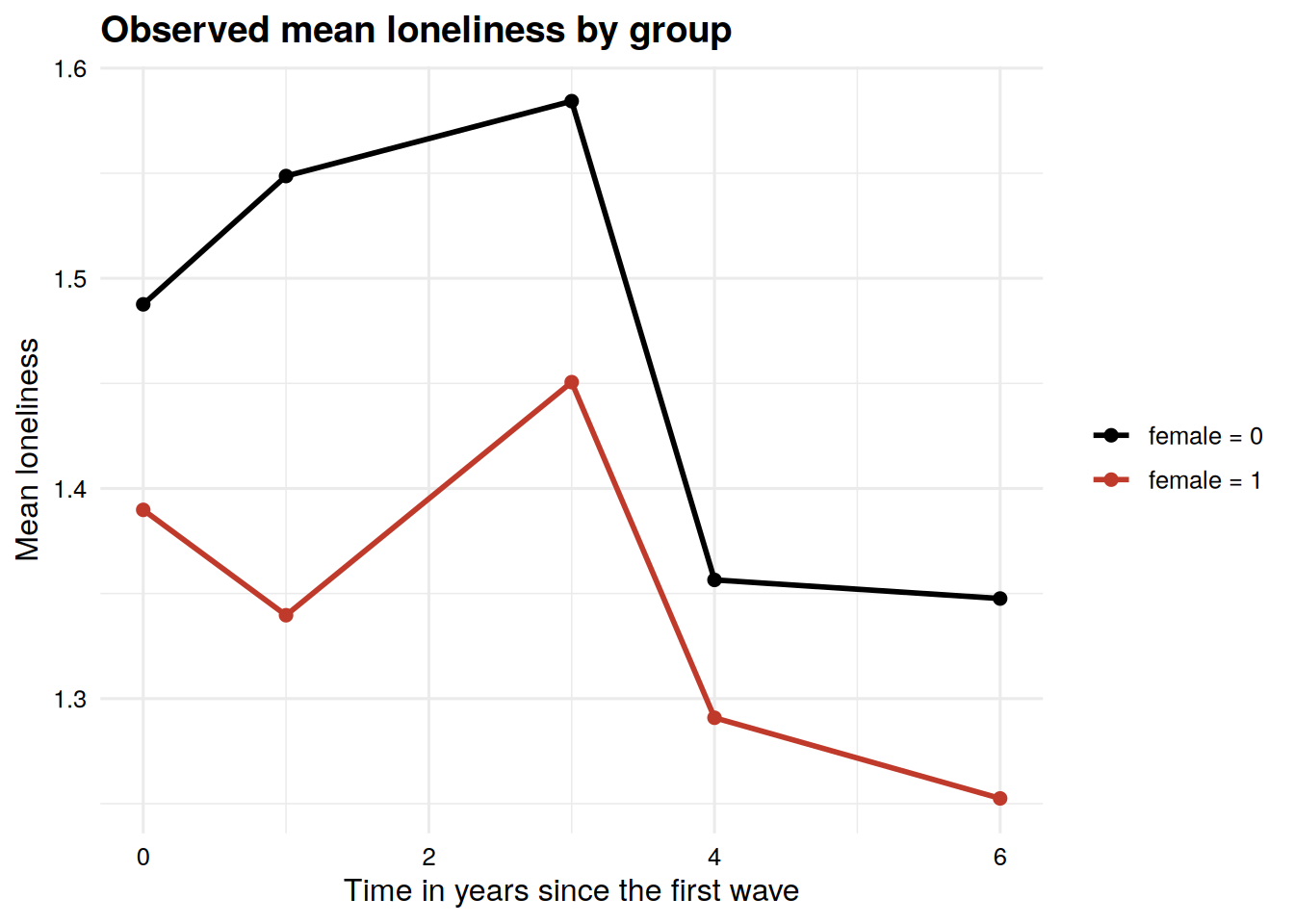
Before fitting anything, it helps to look at the observed means. The plot uses the participants that enter the models, which are those with a non-missing female and complete data on the five loneliness scores.
Code
cc <- data |>filter(!is.na(female), complete.cases(lone1, lone2, lone3, lone4, lone5))n_cc <-table(cc$female)group_means <- cc |>select(female, lone1, lone2, lone3, lone4, lone5) |>pivot_longer(cols =starts_with("lone"), names_to ="wave", values_to ="lone") |>mutate(time =case_match(wave, "lone1"~0, "lone2"~1, "lone3"~3, "lone4"~4, "lone5"~6),group =factor(female, levels =c(0, 1), labels =c("female = 0", "female = 1")) ) |>group_by(group, time) |>summarise(mean_lone =mean(lone), .groups ="drop")ggplot(group_means, aes(x = time, y = mean_lone, color = group, group = group)) +geom_line(linewidth =1) +geom_point(size =2) +scale_color_manual(values =c("black", "#C03A2B")) +labs(x ="Time in years since the first wave", y ="Mean loneliness",color =NULL, title ="Observed mean loneliness by group")
Figure 8.1: Observed mean loneliness at each wave, separately for the two groups. Only participants with complete loneliness data and a non-missing group variable are included.
The plot uses 320 participants, 178 in the group coded 0 and 142 in the group coded 1. The line of the group coded 0 lies above the line of the group coded 1 at all five waves. Notice also that the means do not decline in a perfectly steady way. In both groups the mean at the third wave is higher than at the second wave. A straight line cannot reproduce this pattern.
8.4 The formal model
For participant \(i\) in group \(g\) at wave \(t\), the linear growth model is
The intercept factor \(\eta_0\) and the slope factor \(\eta_1\) have group-specific means \(\alpha_0^{(g)}\) and \(\alpha_1^{(g)}\), variances \(\psi_{00}^{(g)}\) and \(\psi_{11}^{(g)}\), and covariance \(\psi_{01}^{(g)}\). The residual variance \(\theta^{(g)}\) is held equal over the five waves within each group. The four models differ only in which of these group-specific parameters are held equal across the groups.
Table 8.1: The four multigroup models.
Model
Growth factor means
Variances and covariance
Residual variances
Free parameters
Degrees of freedom
M1
equal
equal
equal
6
34
M2
free
equal
equal
8
32
M3
free
free
equal
11
29
M4
free
free
free (equal over time)
12
28
The number of free parameters is the number of estimated parameters minus the number of equality constraints that lavaan reports in its output (20 minus 14, 12, 9 and 8). The two groups provide 20 means and (co)variances each, so the data supply 40 pieces of information in total. The degrees of freedom are 40 minus the number of free parameters.
8.5 Fit the models
All four models use group = "female" in growth(). The labels in c(label1, label2) decide which parameters are held equal. When the same label is used twice, as in c(int, int), the two group-specific parameters are forced to be one number. When two different labels are used, as in c(intm, intf), they are estimated separately.
8.5.1 Model M1, full invariance
Code
multigroupM1 <-' i =~ 1*lone1 + 1*lone2 + 1*lone3 + 1*lone4 + 1*lone5 s =~ 0*lone1 + 1*lone2 + 3*lone3 + 4*lone4 + 6*lone5#Growth factor means constrained equali ~ c(int, int)*1s ~ c(slp, slp)*1#Growth factor variances held equali ~~ c(vint, vint)*is ~~ c(vslp, vslp)*s#Growth factor covariances held equali ~~ c(cvf, cvf)*s#Residual variances of observed items held equallone1 ~~ c(res, res)*lone1lone2 ~~ c(res, res)*lone2lone3 ~~ c(res, res)*lone3lone4 ~~ c(res, res)*lone4lone5 ~~ c(res, res)*lone5'fit_multigroupM1 <-growth(multigroupM1, data = data, group ="female")summary(fit_multigroupM1, fit.measures =TRUE)
lavaan 0.6.17 ended normally after 30 iterations

  Estimator                                         ML
  Optimization method                           NLMINB
  Number of model parameters                        20
  Number of equality constraints                    14

  Number of observations per group:               Used       Total
    0                                              178         222
    1                                              142         193

Model Test User Model:

  Test statistic                               207.477
  Degrees of freedom                                34
  P-value (Chi-square)                           0.000
  Test statistic for each group:
    0                                           98.099
    1                                          109.378

Model Test Baseline Model:

  Test statistic                               463.335
  Degrees of freedom                                20
  P-value                                        0.000

User Model versus Baseline Model:

  Comparative Fit Index (CFI)                    0.609
  Tucker-Lewis Index (TLI)                       0.770

Loglikelihood and Information Criteria:

  Loglikelihood user model (H0)               -776.723
  Loglikelihood unrestricted model (H1)       -672.984

  Akaike (AIC)                                1565.445
  Bayesian (BIC)                              1588.055
  Sample-size adjusted Bayesian (SABIC)       1569.024

Root Mean Square Error of Approximation:

  RMSEA                                          0.179
  90 Percent confidence interval - lower         0.156
  90 Percent confidence interval - upper         0.202
  P-value H_0: RMSEA <= 0.050                    0.000
  P-value H_0: RMSEA >= 0.080                    1.000

Standardized Root Mean Square Residual:

  SRMR                                           0.230

Parameter Estimates:

  Standard errors                             Standard
  Information                                 Expected
  Information saturated (h1) model          Structured


Group 1 [0]:

Latent Variables:
                   Estimate  Std.Err  z-value  P(>|z|)
  i =~
    lone1             1.000
    lone2             1.000
    lone3             1.000
    lone4             1.000
    lone5             1.000
  s =~
    lone1             0.000
    lone2             1.000
    lone3             3.000
    lone4             4.000
    lone5             6.000

Covariances:
                   Estimate  Std.Err  z-value  P(>|z|)
  i ~~
    s        (cvf)   -0.011    0.002   -4.425    0.000

Intercepts:
                   Estimate  Std.Err  z-value  P(>|z|)
    i        (int)    1.484    0.025   60.198    0.000
    s        (slp)   -0.026    0.004   -5.932    0.000

Variances:
                   Estimate  Std.Err  z-value  P(>|z|)
    i       (vint)    0.135    0.016    8.666    0.000
    s       (vslp)    0.001    0.001    2.467    0.014
   .lone1    (res)    0.109    0.005   21.909    0.000
   .lone2    (res)    0.109    0.005   21.909    0.000
   .lone3    (res)    0.109    0.005   21.909    0.000
   .lone4    (res)    0.109    0.005   21.909    0.000
   .lone5    (res)    0.109    0.005   21.909    0.000


Group 2 [1]:

Latent Variables:
                   Estimate  Std.Err  z-value  P(>|z|)
  i =~
    lone1             1.000
    lone2             1.000
    lone3             1.000
    lone4             1.000
    lone5             1.000
  s =~
    lone1             0.000
    lone2             1.000
    lone3             3.000
    lone4             4.000
    lone5             6.000

Covariances:
                   Estimate  Std.Err  z-value  P(>|z|)
  i ~~
    s        (cvf)   -0.011    0.002   -4.425    0.000

Intercepts:
                   Estimate  Std.Err  z-value  P(>|z|)
    i        (int)    1.484    0.025   60.198    0.000
    s        (slp)   -0.026    0.004   -5.932    0.000

Variances:
                   Estimate  Std.Err  z-value  P(>|z|)
    i       (vint)    0.135    0.016    8.666    0.000
    s       (vslp)    0.001    0.001    2.467    0.014
   .lone1    (res)    0.109    0.005   21.909    0.000
   .lone2    (res)    0.109    0.005   21.909    0.000
   .lone3    (res)    0.109    0.005   21.909    0.000
   .lone4    (res)    0.109    0.005   21.909    0.000
   .lone5    (res)    0.109    0.005   21.909    0.000
Notice the warning that the group variable female contains missing values. The 27 rows with a missing group cannot be assigned to a group and are dropped. The table “Number of observations per group” shows that 178 of 222 rows in the group coded 0 and 142 of 193 rows in the group coded 1 are used, so N = 320. The other rows are lost through the listwise deletion of the default settings of growth() (see Chapter 1). Only one of the 27 rows with a missing female had complete loneliness data, which is why N is 320 here and 321 in the earlier chapters.
In M1, the two groups share one intercept mean (1.484), one slope mean (-0.026), one intercept variance (0.135), one slope variance (0.001), one covariance (-0.011), and one residual variance (0.109). The chi-square is 207.477 on 34 degrees of freedom (CFI = .609, RMSEA = .179, SRMR = .230).
8.5.2 Model M2, free growth factor means
Code
multigroupM2 <-' i =~ 1*lone1 + 1*lone2 + 1*lone3 + 1*lone4 + 1*lone5 s =~ 0*lone1 + 1*lone2 + 3*lone3 + 4*lone4 + 6*lone5#Growth factor means freely estimatedi ~ c(intm, intf)*1s ~ c(slpm, slpf)*1#Growth factor variances held equali ~~ c(vint, vint)*is ~~ c(vslp, vslp)*s#Growth factor covariances held equali ~~ c(cvf, cvf)*s#Residual variances of observed items held equallone1 ~~ c(res, res)*lone1lone2 ~~ c(res, res)*lone2lone3 ~~ c(res, res)*lone3lone4 ~~ c(res, res)*lone4lone5 ~~ c(res, res)*lone5'fit_multigroupM2 <-growth(multigroupM2, data = data, group ="female")summary(fit_multigroupM2, fit.measures =TRUE)
lavaan 0.6.17 ended normally after 34 iterations

  Estimator                                         ML
  Optimization method                           NLMINB
  Number of model parameters                        20
  Number of equality constraints                    12

  Number of observations per group:               Used       Total
    0                                              178         222
    1                                              142         193

Model Test User Model:

  Test statistic                               196.543
  Degrees of freedom                                32
  P-value (Chi-square)                           0.000
  Test statistic for each group:
    0                                           94.352
    1                                          102.191

Model Test Baseline Model:

  Test statistic                               463.335
  Degrees of freedom                                20
  P-value                                        0.000

User Model versus Baseline Model:

  Comparative Fit Index (CFI)                    0.629
  Tucker-Lewis Index (TLI)                       0.768

Loglikelihood and Information Criteria:

  Loglikelihood user model (H0)               -771.255
  Loglikelihood unrestricted model (H1)       -672.984

  Akaike (AIC)                                1558.511
  Bayesian (BIC)                              1588.657
  Sample-size adjusted Bayesian (SABIC)       1563.283

Root Mean Square Error of Approximation:

  RMSEA                                          0.179
  90 Percent confidence interval - lower         0.156
  90 Percent confidence interval - upper         0.204
  P-value H_0: RMSEA <= 0.050                    0.000
  P-value H_0: RMSEA >= 0.080                    1.000

Standardized Root Mean Square Residual:

  SRMR                                           0.213

Parameter Estimates:

  Standard errors                             Standard
  Information                                 Expected
  Information saturated (h1) model          Structured


Group 1 [0]:

Latent Variables:
                   Estimate  Std.Err  z-value  P(>|z|)
  i =~
    lone1             1.000
    lone2             1.000
    lone3             1.000
    lone4             1.000
    lone5             1.000
  s =~
    lone1             0.000
    lone2             1.000
    lone3             3.000
    lone4             4.000
    lone5             6.000

Covariances:
                   Estimate  Std.Err  z-value  P(>|z|)
  i ~~
    s        (cvf)   -0.010    0.002   -4.331    0.000

Intercepts:
                   Estimate  Std.Err  z-value  P(>|z|)
    i       (intm)    1.550    0.033   47.589    0.000
    s       (slpm)   -0.031    0.006   -5.236    0.000

Variances:
                   Estimate  Std.Err  z-value  P(>|z|)
    i       (vint)    0.130    0.015    8.547    0.000
    s       (vslp)    0.001    0.001    2.425    0.015
   .lone1    (res)    0.109    0.005   21.909    0.000
   .lone2    (res)    0.109    0.005   21.909    0.000
   .lone3    (res)    0.109    0.005   21.909    0.000
   .lone4    (res)    0.109    0.005   21.909    0.000
   .lone5    (res)    0.109    0.005   21.909    0.000


Group 2 [1]:

Latent Variables:
                   Estimate  Std.Err  z-value  P(>|z|)
  i =~
    lone1             1.000
    lone2             1.000
    lone3             1.000
    lone4             1.000
    lone5             1.000
  s =~
    lone1             0.000
    lone2             1.000
    lone3             3.000
    lone4             4.000
    lone5             6.000

Covariances:
                   Estimate  Std.Err  z-value  P(>|z|)
  i ~~
    s        (cvf)   -0.010    0.002   -4.331    0.000

Intercepts:
                   Estimate  Std.Err  z-value  P(>|z|)
    i       (intf)    1.401    0.036   38.400    0.000
    s       (slpf)   -0.020    0.007   -3.062    0.002

Variances:
                   Estimate  Std.Err  z-value  P(>|z|)
    i       (vint)    0.130    0.015    8.547    0.000
    s       (vslp)    0.001    0.001    2.425    0.015
   .lone1    (res)    0.109    0.005   21.909    0.000
   .lone2    (res)    0.109    0.005   21.909    0.000
   .lone3    (res)    0.109    0.005   21.909    0.000
   .lone4    (res)    0.109    0.005   21.909    0.000
   .lone5    (res)    0.109    0.005   21.909    0.000
Here, the labels of the means change from c(int, int) to c(intm, intf) and from c(slp, slp) to c(slpm, slpf). The intercept means are now 1.550 in the group coded 0 and 1.401 in the group coded 1. The slope means are -0.031 and -0.020. The chi-square is 196.543 on 32 degrees of freedom (CFI = .629, RMSEA = .179, SRMR = .213). The variances, the covariance and the residual variance are still shared by the two groups.
8.5.3 Model M3, free means, variances and covariance
lavaan 0.6.17 ended normally after 82 iterations

  Estimator                                         ML
  Optimization method                           NLMINB
  Number of model parameters                        20
  Number of equality constraints                     9

  Number of observations per group:               Used       Total
    0                                              178         222
    1                                              142         193

Model Test User Model:

  Test statistic                               186.447
  Degrees of freedom                                29
  P-value (Chi-square)                           0.000
  Test statistic for each group:
    0                                           90.667
    1                                           95.780

Model Test Baseline Model:

  Test statistic                               463.335
  Degrees of freedom                                20
  P-value                                        0.000

User Model versus Baseline Model:

  Comparative Fit Index (CFI)                    0.645
  Tucker-Lewis Index (TLI)                       0.755

Loglikelihood and Information Criteria:

  Loglikelihood user model (H0)               -766.208
  Loglikelihood unrestricted model (H1)       -672.984

  Akaike (AIC)                                1554.415
  Bayesian (BIC)                              1595.867
  Sample-size adjusted Bayesian (SABIC)       1560.977

Root Mean Square Error of Approximation:

  RMSEA                                          0.184
  90 Percent confidence interval - lower         0.159
  90 Percent confidence interval - upper         0.210
  P-value H_0: RMSEA <= 0.050                    0.000
  P-value H_0: RMSEA >= 0.080                    1.000

Standardized Root Mean Square Residual:

  SRMR                                           0.177

Parameter Estimates:

  Standard errors                             Standard
  Information                                 Expected
  Information saturated (h1) model          Structured


Group 1 [0]:

Latent Variables:
                   Estimate  Std.Err  z-value  P(>|z|)
  i =~
    lone1             1.000
    lone2             1.000
    lone3             1.000
    lone4             1.000
    lone5             1.000
  s =~
    lone1             0.000
    lone2             1.000
    lone3             3.000
    lone4             4.000
    lone5             6.000

Covariances:
                   Estimate  Std.Err  z-value  P(>|z|)
  i ~~
    s       (covm)   -0.015    0.004   -4.140    0.000

Intercepts:
                   Estimate  Std.Err  z-value  P(>|z|)
    i       (intm)    1.550    0.036   43.187    0.000
    s       (slpm)   -0.031    0.006   -4.949    0.000

Variances:
                   Estimate  Std.Err  z-value  P(>|z|)
    i       (vinm)    0.170    0.024    6.957    0.000
    s       (vslm)    0.002    0.001    2.662    0.008
   .lone1    (res)    0.109    0.005   21.909    0.000
   .lone2    (res)    0.109    0.005   21.909    0.000
   .lone3    (res)    0.109    0.005   21.909    0.000
   .lone4    (res)    0.109    0.005   21.909    0.000
   .lone5    (res)    0.109    0.005   21.909    0.000


Group 2 [1]:

Latent Variables:
                   Estimate  Std.Err  z-value  P(>|z|)
  i =~
    lone1             1.000
    lone2             1.000
    lone3             1.000
    lone4             1.000
    lone5             1.000
  s =~
    lone1             0.000
    lone2             1.000
    lone3             3.000
    lone4             4.000
    lone5             6.000

Covariances:
                   Estimate  Std.Err  z-value  P(>|z|)
  i ~~
    s       (covf)   -0.004    0.003   -1.484    0.138

Intercepts:
                   Estimate  Std.Err  z-value  P(>|z|)
    i       (intf)    1.401    0.031   44.901    0.000
    s       (slpf)   -0.020    0.006   -3.321    0.001

Variances:
                   Estimate  Std.Err  z-value  P(>|z|)
    i       (vinf)    0.079    0.017    4.753    0.000
    s       (vslf)    0.000    0.001    0.569    0.569
   .lone1    (res)    0.109    0.005   21.909    0.000
   .lone2    (res)    0.109    0.005   21.909    0.000
   .lone3    (res)    0.109    0.005   21.909    0.000
   .lone4    (res)    0.109    0.005   21.909    0.000
   .lone5    (res)    0.109    0.005   21.909    0.000
The intercept variance is now 0.170 in the group coded 0 and 0.079 in the group coded 1. The slope variances are very small in both groups (0.002 and 0.000), and in the group coded 1 the slope variance is not distinguishable from zero (p = .569). The covariance between the intercept and the slope is -0.015 in the group coded 0 (p < .001) and -0.004 in the group coded 1 (p = .138). The chi-square is 186.447 on 29 degrees of freedom (CFI = .645, RMSEA = .184, SRMR = .177).
8.5.4 Model M4, free residual variances
Code
multigroupM4 <-' i =~ 1*lone1 + 1*lone2 + 1*lone3 + 1*lone4 + 1*lone5 s =~ 0*lone1 + 1*lone2 + 3*lone3 + 4*lone4 + 6*lone5#Growth factor means freely estimatedi ~ c(intm, intf)*1s ~ c(slpm, slpf)*1#Growth factor variances freely estimatedi ~~ c(vinm, vinf)*is ~~ c(vslm, vslf)*s#Growth factor covariances freely estimatedi ~~ c(covm, covf)*s#Residual variances of observed items freely estimated across groups but held equal over time in groupslone1 ~~ c(rsm, rsf)*lone1lone2 ~~ c(rsm, rsf)*lone2lone3 ~~ c(rsm, rsf)*lone3lone4 ~~ c(rsm, rsf)*lone4lone5 ~~ c(rsm, rsf)*lone5'fit_multigroupM4 <-growth(multigroupM4, data = data, group ="female")summary(fit_multigroupM4, fit.measures =TRUE)
lavaan 0.6.17 ended normally after 49 iterations

  Estimator                                         ML
  Optimization method                           NLMINB
  Number of model parameters                        20
  Number of equality constraints                     8

  Number of observations per group:               Used       Total
    0                                              178         222
    1                                              142         193

Model Test User Model:

  Test statistic                               178.403
  Degrees of freedom                                28
  P-value (Chi-square)                           0.000
  Test statistic for each group:
    0                                           87.439
    1                                           90.964

Model Test Baseline Model:

  Test statistic                               463.335
  Degrees of freedom                                20
  P-value                                        0.000

User Model versus Baseline Model:

  Comparative Fit Index (CFI)                    0.661
  Tucker-Lewis Index (TLI)                       0.758

Loglikelihood and Information Criteria:

  Loglikelihood user model (H0)               -762.185
  Loglikelihood unrestricted model (H1)       -672.984

  Akaike (AIC)                                1548.371
  Bayesian (BIC)                              1593.591
  Sample-size adjusted Bayesian (SABIC)       1555.529

Root Mean Square Error of Approximation:

  RMSEA                                          0.183
  90 Percent confidence interval - lower         0.158
  90 Percent confidence interval - upper         0.209
  P-value H_0: RMSEA <= 0.050                    0.000
  P-value H_0: RMSEA >= 0.080                    1.000

Standardized Root Mean Square Residual:

  SRMR                                           0.172

Parameter Estimates:

  Standard errors                             Standard
  Information                                 Expected
  Information saturated (h1) model          Structured


Group 1 [0]:

Latent Variables:
                   Estimate  Std.Err  z-value  P(>|z|)
  i =~
    lone1             1.000
    lone2             1.000
    lone3             1.000
    lone4             1.000
    lone5             1.000
  s =~
    lone1             0.000
    lone2             1.000
    lone3             3.000
    lone4             4.000
    lone5             6.000

Covariances:
                   Estimate  Std.Err  z-value  P(>|z|)
  i ~~
    s       (covm)   -0.014    0.004   -3.668    0.000

Intercepts:
                   Estimate  Std.Err  z-value  P(>|z|)
    i       (intm)    1.550    0.036   43.187    0.000
    s       (slpm)   -0.031    0.006   -4.949    0.000

Variances:
                   Estimate  Std.Err  z-value  P(>|z|)
    i       (vinm)    0.163    0.025    6.632    0.000
    s       (vslm)    0.001    0.001    1.842    0.065
   .lone1    (rsm)    0.121    0.007   16.340    0.000
   .lone2    (rsm)    0.121    0.007   16.340    0.000
   .lone3    (rsm)    0.121    0.007   16.340    0.000
   .lone4    (rsm)    0.121    0.007   16.340    0.000
   .lone5    (rsm)    0.121    0.007   16.340    0.000


Group 2 [1]:

Latent Variables:
                   Estimate  Std.Err  z-value  P(>|z|)
  i =~
    lone1             1.000
    lone2             1.000
    lone3             1.000
    lone4             1.000
    lone5             1.000
  s =~
    lone1             0.000
    lone2             1.000
    lone3             3.000
    lone4             4.000
    lone5             6.000

Covariances:
                   Estimate  Std.Err  z-value  P(>|z|)
  i ~~
    s       (covf)   -0.006    0.003   -2.146    0.032

Intercepts:
                   Estimate  Std.Err  z-value  P(>|z|)
    i       (intf)    1.401    0.031   44.901    0.000
    s       (slpf)   -0.020    0.006   -3.321    0.001

Variances:
                   Estimate  Std.Err  z-value  P(>|z|)
    i       (vinf)    0.087    0.017    5.217    0.000
    s       (vslf)    0.001    0.001    1.565    0.118
   .lone1    (rsf)    0.093    0.006   14.595    0.000
   .lone2    (rsf)    0.093    0.006   14.595    0.000
   .lone3    (rsf)    0.093    0.006   14.595    0.000
   .lone4    (rsf)    0.093    0.006   14.595    0.000
   .lone5    (rsf)    0.093    0.006   14.595    0.000
In M4, the residual variance is 0.121 in the group coded 0 and 0.093 in the group coded 1. The intercept variances change slightly compared with M3 (0.163 and 0.087), and the covariances become -0.014 (p < .001) and -0.006 (p = .032). The slope variances are 0.001 and 0.001, with p = .065 and p = .118. The chi-square is 178.403 on 28 degrees of freedom (CFI = .661, RMSEA = .183, SRMR = .172).
Besides the warning about the missing values in female, lavaan gave no warning for the four models, although the slope variances are close to zero.
8.6 Understanding the output
8.6.1 Fit of the four models
The fit indexes of the four models are collected in Table 8.2. The code that builds the table is not part of the workshop.
Table 8.2: Fit of the four multigroup models (listwise deletion, N = 320).
Model
Chi-square
df
CFI
TLI
RMSEA
SRMR
AIC
BIC
M1
207.477
34
0.609
0.770
0.179
0.230
1565.4
1588.1
M2
196.543
32
0.629
0.768
0.179
0.213
1558.5
1588.7
M3
186.447
29
0.645
0.755
0.184
0.177
1554.4
1595.9
M4
178.403
28
0.661
0.758
0.183
0.172
1548.4
1593.6
All four models fit poorly. The chi-square tests are significant, the CFI values lie between .609 and .661, the TLI values between .755 and .770, and the RMSEA values are about .18 with lower confidence limits above .15. The test of close fit and the test of not-close fit confirm this: the p value for the hypothesis that the RMSEA is at most .05 is .000, and the p value for the hypothesis that it is at least .08 is 1.000. These values are far from the usual cut-offs of a CFI of about .95 or more and an RMSEA of about .06 or less (Hu & Bentler, 1999).
The SRMR is high in all four models. It is .230 for M1 and decreases to .172 for M4. The SRMR summarizes the differences between the observed and the model-implied means and covariances, and values below about .08 are usually taken as good (Hu & Bentler, 1999). A value of .172 for the least constrained model suggests that the linear growth model with constant residual variances does not reproduce the observed means and covariances well, whichever of the four constraint sets we use. The decrease from M1 to M4 shows that freeing parameters by group reduces the misfit. It does not remove it.
To see where the misfit comes from, we compare the observed means and variances with those implied by M4. This is an addition to the workshop.
Code
# Addition, not part of the workshopimp <-fitted(fit_multigroupM4)obs_m <- cc |>group_by(female) |>summarise(across(lone1:lone5, list(m = mean, v = var)), .groups ="drop")misfit <-do.call(rbind, lapply(1:2, function(g) { gcode <-c(0, 1)[g] o <- obs_m[obs_m$female == gcode, ]data.frame(Group =paste("female =", gcode), Wave =1:5,Time =c(0, 1, 3, 4, 6),Observed_mean =unlist(o[paste0("lone", 1:5, "_m")]),Implied_mean =as.numeric(imp[[g]]$mean),Observed_var =unlist(o[paste0("lone", 1:5, "_v")]),Implied_var =diag(imp[[g]]$cov))}))knitr::kable(misfit, digits =3, row.names =FALSE)
Table 8.3: Observed and model-implied means and variances of the five loneliness scores under M4, by group (listwise deletion).
Group
Wave
Time
Observed_mean
Implied_mean
Observed_var
Implied_var
female = 0
1
0
1.488
1.550
0.208
0.285
female = 0
2
1
1.549
1.520
0.315
0.259
female = 0
3
3
1.584
1.459
0.264
0.215
female = 0
4
4
1.356
1.428
0.191
0.197
female = 0
5
6
1.348
1.367
0.130
0.171
female = 1
1
0
1.390
1.401
0.147
0.181
female = 1
2
1
1.340
1.381
0.156
0.170
female = 1
3
3
1.451
1.341
0.251
0.154
female = 1
4
4
1.291
1.321
0.133
0.150
female = 1
5
6
1.253
1.281
0.104
0.147
In both groups, the implied means decrease in a straight line, while the observed means go up from the second to the third wave and then fall. In the group coded 0, the observed variance rises from 0.208 at the first wave to 0.315 at the second wave and then falls to 0.130 at the fifth wave, whereas the implied variance falls steadily from 0.285 to 0.171. Thus, both the linear mean structure and the constant residual variance over time are likely candidates for the poor fit. We do not test this explanation here. It suggests that the model of the earlier chapters should be revised before any group comparison is taken as substantive.
The loneliness scores are also skewed (see Chapter 1 for the consequences). As a check, we refit the four models with the robust maximum likelihood estimator MLR (Yuan & Bentler, 2000). This is an addition to the workshop.
Code
# Addition, not part of the workshoprob <-sapply(list(multigroupM1, multigroupM2, multigroupM3, multigroupM4), function(m)fitMeasures(growth(m, data = data, group ="female", estimator ="MLR"),c("cfi.robust", "rmsea.robust")))sk <- psych::describe(cc[paste0("lone", 1:5)])
In the participants of the models, the skewness of the five scores ranges from 1.5 to 2.7 and the kurtosis reaches 9.6. The robust CFI is between .690 and .724 and the robust RMSEA between .154 and .161 for the four models. The robust indexes remain poor, so non-normality alone does not explain the misfit.
8.6.2 Estimates
The estimates of the models are in the output above. Remember that one time unit is one year, so the slope means are changes per year, and that the intercept is the expected loneliness score at the first wave. In M4, the intercept mean is 1.550 in the group coded 0 and 1.401 in the group coded 1. The slope mean is -0.031 and -0.020, respectively. The decline is estimated as steeper in the group coded 0, but this difference is small compared with its standard error, as the Wald test below shows.
8.7 Compare the models
8.7.1 Chi-square difference tests
The function anova() compares the four models in one call. Because the models are nested, each model is compared with the next less constrained model.
lavaan orders the table from the model with the fewest degrees of freedom (M4) to the model with the most (M1). The columns “Chisq diff”, “Df diff” and “Pr(>Chisq)” in each row compare that row with the row above it. Reading from the bottom of the table upward, we obtain the three steps of the sequence. The chi-square difference test compares two nested models through the difference of their chi-square values (Bentler & Bonett, 1980).
M1 versus M2: the chi-square difference is 10.934 on 2 degrees of freedom (p = .004).
M2 versus M3: the chi-square difference is 10.096 on 3 degrees of freedom (p = .018).
M3 versus M4: the chi-square difference is 8.044 on 1 degree of freedom (p = .005).
A significant chi-square difference means that the reduced model is rejected, so the model with more free parameters fits better. All three differences are significant at the .05 level. This holds only if the less constrained model is itself correct, and the CFI of .61 to .66 says that it is not. The three tests are therefore not clean evidence that the groups differ. The M2 versus M3 test frees the slope variances, and these are at or near zero, the boundary of the parameter space. The reference chi-square distribution is then a mixture and the p value of .018 is only approximate (Self & Liang, 1987). The sequence also depends on its order, because M1 versus M2 is tested while the variances are held equal. The Wald tests on M4 below test one parameter at a time.
The AIC (Akaike, 1974) points in the same direction as the chi-square differences and is lowest for M4 (1548.4). The BIC (Schwarz, 1978) does not agree. It is lowest for M1 (1588.1) and nearly the same for M2 (1588.7), and it is higher for M3 (1595.9) and M4 (1593.6). The BIC penalizes additional parameters more strongly than the AIC, so it favors the more constrained models.
8.7.2 The workshop slides
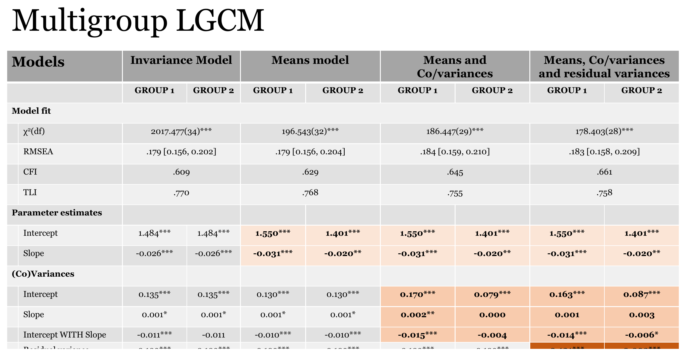
Figure 8.2 and Figure 8.3 show the two slides of the workshop for this chapter. The slides display Mplus estimates. The numbers in this chapter are the ones from the R output, and the two sets agree closely for the estimates and the fit indexes.
Figure 8.2: Results of the four multigroup models as shown on the workshop slide (Mplus estimates). Source: workshop slides (Anyan, 2023).
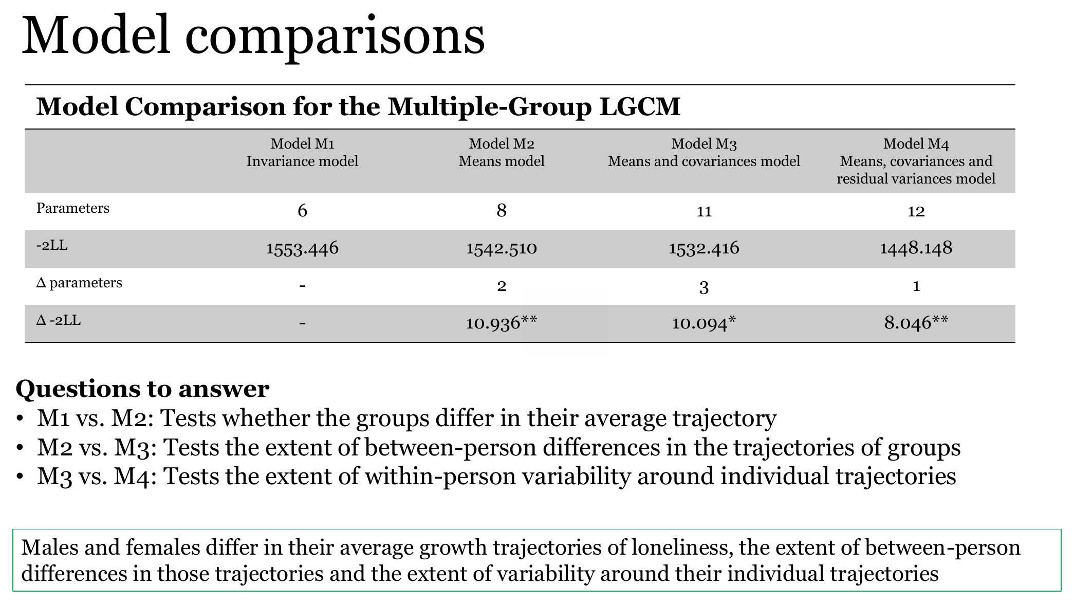
The comparison slide reports the difference in -2LL, which is -2 times the loglikelihood, whereas anova() reports chi-square differences. For models fitted to the same data, the two are the same quantity up to rounding. The values from anova() are 10.934, 10.096 and 8.044, and the values on the slide are 10.936, 10.094 and 8.046. In this chapter we use the chi-square differences from R. Two entries of the slide tables differ from the R output. The slide prints the chi-square of M1 as 2017.477, whereas R gives 207.477. It prints the -2LL of M4 as 1448.148, whereas R gives 1524.370 (-2 times -762.185), which is consistent with the printed difference of 8.046 from M3. The slide also gives 0.003 for the slope variance of the second group in M4, whereas R gives 0.001.
Figure 8.3: Model comparison and the three questions of the sequence as shown on the workshop slide (Mplus estimates). Source: workshop slides (Anyan, 2023).
The slide concludes that the groups differ in their average growth trajectories, in the extent of between-person differences in those trajectories, and in the extent of variability around the individual trajectories. This is what the three difference tests say, taken at face value, and the caveats above apply to it.
Compare models only when the fit is acceptable
Only models with acceptable fit should be compared substantively. A significant chi-square difference between two nested models says that the more complex model fits better than the simpler one. It does not say that the more complex model fits the data well. Here all four models have a CFI between .609 and .661. The tests tell us how the misfit changes when parameters are freed, and the answer applies only as long as the common linear structure is assumed to be correct. When it is not, a significant difference may reflect the misspecification instead of a real difference between the groups.
8.7.3 Differences in fit indexes
A rule of thumb from invariance testing is to look at the change in CFI between models (Cheung & Rensvold, 2002). A decrease of .01 or more is usually taken to indicate a worse fit for the constrained model. The CFI increases by .020 from M1 to M2, by .016 from M2 to M3, and by .016 from M3 to M4. This is in the same direction as the chi-square difference tests. The rule was developed for measurement invariance and we apply it here only by analogy. All of the CFI values remain far below the usual cut-offs.
8.8 Test single parameters with Wald tests
The three tests above each bundle several parameters. The M1 versus M2 test has 2 degrees of freedom and so it cannot say whether the intercept mean, the slope mean, or both differ between the groups. The same applies to the 3-degree-of-freedom test of M2 versus M3. To test one parameter at a time, we use Wald tests on M4, the model in which all six parameters are free and carry separate labels for the two groups. The likelihood ratio test and the Wald test are two asymptotically equivalent ways of testing a constraint (Buse, 1982). With lavTestWald(), we test the null hypothesis that the difference between the two labeled parameters is zero. Each test has one degree of freedom.
Code
#Test significant difference between groups in the intercept growth factorconstint ='intm - intf == 0'lavTestWald(fit_multigroupM4, constraints = constint)
#Test significant difference between groups in the variability around interceptconstint_var ='vinm - vinf == 0'lavTestWald(fit_multigroupM4, constraints = constint_var)
#Test significant difference between groups in the variability around slopeconstslp_var ='vslm - vslf == 0'lavTestWald(fit_multigroupM4, constraints = constslp_var)
#Test significant difference between groups in the variability around the relationship between intercept and slopeconstslp_cov_var ='covm - covf == 0'lavTestWald(fit_multigroupM4, constraints = constslp_cov_var)
#Test significant difference between groups in the residual variabilityconstslp_res_var ='rsm - rsf == 0'lavTestWald(fit_multigroupM4, constraints = constslp_res_var)
Table 8.4 collects the six tests together with the estimates of M4 for the two groups.
Table 8.4: Wald tests of the group differences in M4 (listwise deletion, N = 320).
Parameter
Group coded 0
Group coded 1
Constraint
Wald chi-square (1)
p
Intercept mean
1.550
1.401
intm - intf == 0
9.912
.002
Slope mean
-0.031
-0.020
slpm - slpf == 0
1.495
.221
Intercept variance
0.163
0.087
vinm - vinf == 0
6.503
.011
Slope variance
0.001
0.001
vslm - vslf == 0
0.150
.699
Covariance
-0.014
-0.006
covm - covf == 0
2.798
.094
Residual variance
0.121
0.093
rsm - rsf == 0
8.154
.004
Three of the six differences are significant at the .05 level: the intercept mean, the intercept variance, and the residual variance. The slope mean, the slope variance, and the covariance do not differ significantly. The covariance is close to the .05 level (p = .094).
Six tests were run on the same model. If we divided the .05 level by six (.0083, a Bonferroni-type correction), the intercept mean and the residual variance would remain significant, whereas the intercept variance (p = .011) would not. We mention this as a reminder that the intercept variance is the weakest of the three results, not as a rule that was followed in the workshop.
The slope variances in M4 are 0.001 in both groups, with standard errors of the same size, and the variance of a latent factor cannot be below zero. Close to this boundary of the parameter space, the normal approximation behind the Wald test is not reliable. The test for the slope variance should therefore be read as showing no evidence of a group difference, and not as showing that the two slope variances are equal.
8.9 Sensitivity to the missing data handling
The workshop script uses growth() with its default settings, so the models above rest on the 320 participants with complete loneliness data and a non-missing female (Chapter 1). As a check, we refit the four models with missing = "fiml". The syntax of the models is the same as before. This section is an addition to the workshop.
Code
# Addition, not part of the workshopfit_fiml <-lapply(list(M1 = multigroupM1, M2 = multigroupM2,M3 = multigroupM3, M4 = multigroupM4),function(m) growth(m, data = data, group ="female", missing ="fiml"))n_fiml <-lavInspect(fit_fiml$M4, "nobs")fiml_tab <-t(sapply(fit_fiml, function(f)fitMeasures(f, c("chisq", "df", "cfi", "tli", "rmsea", "srmr", "aic", "bic"))))fiml_tab <-data.frame(Model =rownames(fiml_tab), fiml_tab, row.names =NULL)names(fiml_tab) <-c("Model", "Chi-square", "df", "CFI", "TLI", "RMSEA", "SRMR", "AIC", "BIC")knitr::kable(fiml_tab, digits =c(0, 3, 0, 3, 3, 3, 3, 1, 1),caption ="Fit of the four multigroup models with FIML.")
Fit of the four multigroup models with FIML.
Model
Chi-square
df
CFI
TLI
RMSEA
SRMR
AIC
BIC
M1
186.324
34
0.711
0.830
0.147
0.218
2037.0
2061.1
M2
171.986
32
0.735
0.834
0.146
0.200
2026.6
2058.8
M3
153.852
29
0.763
0.837
0.145
0.142
2014.5
2058.7
M4
144.694
28
0.779
0.842
0.142
0.138
2007.4
2055.6
lavaan again warns about the missing values in the group variable. It also reports that three rows are empty, meaning that they have no observed loneliness score at all, and ignores them. The 27 rows with a missing female still cannot be used. As a result, N is 412 (222 and 190) instead of 320. The fit improves but remains poor, with CFI between .711 and .779 and RMSEA between .142 and .147. The sequence of difference tests and the group differences can be checked in the same way.
Code
# Addition, not part of the workshopcg_fiml <-anova(fit_fiml$M1, fit_fiml$M2, fit_fiml$M3, fit_fiml$M4)cg_fiml
Estimates of M4 with listwise deletion and with FIML, and the Wald tests under FIML.
Parameter
Group0_listwise
Group0_FIML
Group1_listwise
Group1_FIML
Wald
p
Intercept mean
1.550
1.569
1.401
1.403
13.86
0.000
Slope mean
-0.031
-0.034
-0.020
-0.020
2.93
0.087
Intercept variance
0.163
0.189
0.087
0.092
10.72
0.001
Slope variance
0.001
0.002
0.001
0.001
2.06
0.151
Covariance
-0.014
-0.017
-0.006
-0.005
6.34
0.012
Residual variance
0.121
0.125
0.093
0.097
9.17
0.002
The estimates change little. The intercept mean of the group coded 0 changes from 1.550 to 1.569, and that of the group coded 1 from 1.401 to 1.403. The slope mean of the group coded 0 changes from -0.031 to -0.034, and that of the group coded 1 stays at -0.020. The variances are somewhat larger under FIML, for example 0.163 and 0.189 for the intercept variance in the group coded 0. The three chi-square difference tests remain significant under FIML (14.338 on 2 degrees of freedom for M1 versus M2, 18.134 on 3 for M2 versus M3, and 9.158 on 1 for M3 versus M4). The Wald tests lead to the same conclusion for the intercept mean (p < .001), the intercept variance (p = .001), the residual variance (p = .002), the slope mean (p = .087) and the slope variance (p = .151). The covariance is the exception. Its difference is not significant under listwise deletion (p = .094) and is significant under FIML (p = .012). The conclusion about the covariance therefore depends on how the missing data are handled and should be reported with this caveat.
8.10 Interpretation
The group coded 0 has a higher average level of loneliness at the first wave (1.550 against 1.401), more variation between participants in that level (0.163 against 0.087), and more residual variance around the individual lines (0.121 against 0.093). The average slopes are both slightly negative (-0.031 and -0.020 per year), and there is no clear evidence in these data that the average rate of change differs between the groups. The variance of the slope is estimated close to zero in both groups, so the groups hardly differ in how much the rate of change varies from person to person, as far as this model can show.
These statements are tied to the models and to what they assume. The four models fit poorly by every index we looked at, and freeing the group constraints reduces the misfit only a little. The observed means do not follow a straight line and the observed variances change across the waves. Under these conditions, the chi-square differences, the AIC, and the Wald tests describe the relative fit and the group differences of a linear model that does not fit either group well. The pattern of the differences is consistent across the listwise and FIML analyses, with the exception of the covariance. Still, we should treat it as a description of this model and not as a firm statement about how the groups differ. It is also not possible, with these data, to say why the groups differ. The models contain no explanatory variables.
8.11 What changed compared with the previous model
In Chapter 7, one growth model was fitted to all participants and the factors predicted a distal outcome. Here, there is no outcome. The growth model stays the same, and the new element is the grouping variable. Instead of one set of growth parameters, there is one set per group, and the question moves from what the growth factors predict to whether the growth factors differ between the groups. The four models are compared with a sequence of nested tests in one anova() call. The restriction that the residual variance is equal over time, used for all four models, is a simplification that the observed variances in Table 8.3 do not support well.
Compared with using the grouping variable as a covariate of the intercept and the slope (Chapter 5), the multigroup approach lets the variances, the covariance and the residual variances differ by group, and not only the means.
8.12 What this model answers and what it cannot tell
The multigroup sequence answers whether the average trajectory, the between-person differences in the trajectory, and the residual variability can be held equal across two groups. The Wald tests narrow this down to single parameters. In this dataset, the tests suggest that the groups differ in the intercept mean, the intercept variance and the residual variance, and that there is no clear evidence for differences in the slope mean and the slope variance.
The sequence cannot tell us how the groups differ in anything the linear model does not describe, such as the bend in the observed means. It cannot tell us why the groups differ. It does not test the equality of the loadings, because the time scores are fixed and identical across the groups. Because the model fit is poor, the answer is a limited one. The sequence also compares only the two groups defined by one variable and the tests can be affected by the near-zero slope variances, the non-normality, and the loss of rows through listwise deletion.
8.13 Researcher’s perspective
Start with the single-group model in each group, or with the pooled model, and examine whether it fits before moving to the group comparison. Here, the pooled linear model already fits poorly (see Chapter 2), and the multigroup models inherit this problem. A better strategy would be to improve the shape of the growth model first, for instance with the piecewise models of Chapter 3, and then to repeat the sequence M1 to M4.
Report the group coding and the number of participants in each group (178 and 142 in the listwise analysis), the rows lost because of missing values on female, and the missing data handling. Report the fit of every model and not only the chi-square difference tests. Report which test statistic was used for the comparison, here the chi-square difference from anova(). When a robust estimator is used for non-normal data, the differences should be tested with a scaled chi-square difference (Satorra & Bentler, 2001). Decide in advance which parameters you will test. The six Wald tests here follow the six parameters of the growth model, and each of them is a separate test. Where the answer depends on the missing data handling, as for the covariance, say so.
Akaike, H. (1974). A new look at the statistical model identification. IEEE Transactions on Automatic Control, 19(6), 716–723. https://doi.org/10.1109/TAC.1974.1100705
Anyan, F. (2023). Longitudinal data analysis using Mplus and R. Workshop slides.
Bentler, P. M., & Bonett, D. G. (1980). Significance tests and goodness of fit in the analysis of covariance structures. Psychological Bulletin, 88(3), 588–606. https://doi.org/10.1037/0033-2909.88.3.588
Buse, A. (1982). The likelihood ratio, Wald, and Lagrange multiplier tests: An expository note. The American Statistician, 36(3a), 153–157. https://doi.org/10.1080/00031305.1982.10482817
Cheung, G. W., & Rensvold, R. B. (2002). Evaluating goodness-of-fit indexes for testing measurement invariance. Structural Equation Modeling: A Multidisciplinary Journal, 9(2), 233–255.
Hu, L., & Bentler, P. M. (1999). Cutoff criteria for fit indexes in covariance structure analysis: Conventional criteria versus new alternatives. Structural Equation Modeling: A Multidisciplinary Journal, 6(1), 1–55. https://doi.org/10.1080/10705519909540118
Satorra, A., & Bentler, P. M. (2001). A scaled difference chi-square test statistic for moment structure analysis. Psychometrika, 66(4), 507–514. https://doi.org/10.1007/BF02296192
Schwarz, G. (1978). Estimating the dimension of a model. The Annals of Statistics, 6(2), 461–464.
Self, S. G., & Liang, K.-Y. (1987). Asymptotic properties of maximum likelihood estimators and likelihood ratio tests under nonstandard conditions. Journal of the American Statistical Association, 82(398), 605–610. https://doi.org/10.1080/01621459.1987.10478472
Yuan, K.-H., & Bentler, P. M. (2000). Three likelihood-based methods for mean and covariance structure analysis with nonnormal missing data. Sociological Methodology, 30, 165–200.
Source Code
# Multigroup growth models {#sec-multigroup}```{r}#| label: setup#| include: falselibrary(lavaan)library(dplyr)library(tidyr)library(ggplot2)library(psych)data <-read.csv("data/data.csv", fileEncoding ="UTF-8-BOM")# Helpers for the inline numbers in the textcf <-function(f, k) sprintf("%.3f", coef(f)[[k]])pf <-function(p) ifelse(p < .001, "< .001", paste0("= ", sub("^0", "", sprintf("%.3f", p))))dd <-function(x) sub("^0", "", sprintf("%.3f", x))fi <-function(f) { m <-fitMeasures(f, c("chisq", "df", "cfi", "rmsea", "srmr"))sprintf("chi-square is %.3f on %d degrees of freedom (CFI = %s, RMSEA = %s, SRMR = %s)", m[["chisq"]], as.integer(m[["df"]]), dd(m[["cfi"]]), dd(m[["rmsea"]]), dd(m[["srmr"]]))}theme_set(theme_minimal(base_size =12) +theme(plot.title =element_text(face ="bold", color ="black"),axis.title =element_text(color ="black"),axis.text =element_text(color ="black"),strip.text =element_text(color ="black"),legend.text =element_text(color ="black"),legend.title =element_text(color ="black"),plot.caption =element_text(color ="black")))```## Why compare groupsThe models in the previous chapters describe one growth process for all participants in the dataset. In @sec-distal we asked what the initial level and the rate of change of loneliness predict. A different question is whether the growth process is the same in two groups. Here, we ask whether the initial level, the rate of change and the between-person variation are equal in the two groups. A *multigroup growth model* answers this by fitting the same growth model in each group at the same time and by testing which parameters can be held equal across the groups.A multiple-group approach to growth models is described in @duncan2004introduction. In the workshop, we used the grouping variable `female`, which has the values 0 and 1 in the dataset. This chapter follows that analysis. We start with a model in which everything is held equal across the groups and then free one block of parameters at a time.## The idea in plain languageThe growth model has a few parameters: the means of the intercept factor and the slope factor, their variances, their covariance and the residual variance. Holding these parameters equal across the groups says that one set of values describes both groups. Freeing them says that each group has its own set.The models are built in four steps, and every step is nested in the one before it.- *M1* holds everything equal: growth factor means, growth factor variances and covariance, and residual variances.- *M2* frees the growth factor means.- *M3* also frees the growth factor variances and the covariance.- *M4* also frees the residual variances, which are still held equal over time within each group.M1 versus M2 tests whether the groups differ in their average trajectory. M2 versus M3 tests the extent of between-person differences in the trajectories of the groups. M3 versus M4 tests the extent of within-person variability around the individual trajectories. These are the three questions on the workshop slide in @fig-multigroup-comparison-slide.## A concrete exampleWe use the five loneliness scores (`lone1` to `lone5`) and the time scores 0, 1, 3, 4 and 6, as in the earlier chapters. The grouping variable is `female`. In the dataset, 222 rows are coded 0, 193 rows are coded 1, and 27 rows have a missing value. The workshop slides call the two groups male and female. Here, we refer to them by their codes. The output of lavaan labels the first group as "Group 1 [0]" and the second as "Group 2 [1]", and the labels `m` and `f` in the syntax follow this order. Thus, `m` belongs to the group coded 0 and `f` to the group coded 1.Before fitting anything, it helps to look at the observed means. The plot uses the participants that enter the models, which are those with a non-missing `female` and complete data on the five loneliness scores.```{r}#| label: fig-group-means#| fig-cap: "Observed mean loneliness at each wave, separately for the two groups. Only participants with complete loneliness data and a non-missing group variable are included."#| fig-alt: "Line plot of the observed mean loneliness score against time in years for the group coded 0 and the group coded 1"cc <- data |>filter(!is.na(female), complete.cases(lone1, lone2, lone3, lone4, lone5))n_cc <-table(cc$female)group_means <- cc |>select(female, lone1, lone2, lone3, lone4, lone5) |>pivot_longer(cols =starts_with("lone"), names_to ="wave", values_to ="lone") |>mutate(time =case_match(wave, "lone1"~0, "lone2"~1, "lone3"~3, "lone4"~4, "lone5"~6),group =factor(female, levels =c(0, 1), labels =c("female = 0", "female = 1")) ) |>group_by(group, time) |>summarise(mean_lone =mean(lone), .groups ="drop")ggplot(group_means, aes(x = time, y = mean_lone, color = group, group = group)) +geom_line(linewidth =1) +geom_point(size =2) +scale_color_manual(values =c("black", "#C03A2B")) +labs(x ="Time in years since the first wave", y ="Mean loneliness",color =NULL, title ="Observed mean loneliness by group")```The plot uses `r nrow(cc)` participants, `r n_cc[["0"]]` in the group coded 0 and `r n_cc[["1"]]` in the group coded 1. The line of the group coded 0 lies above the line of the group coded 1 at all five waves. Notice also that the means do not decline in a perfectly steady way. In both groups the mean at the third wave is higher than at the second wave. A straight line cannot reproduce this pattern.## The formal modelFor participant $i$ in group $g$ at wave $t$, the linear growth model is$$y_{ti}^{(g)} = \eta_{0i}^{(g)} + \lambda_t \, \eta_{1i}^{(g)} + \varepsilon_{ti}^{(g)}, \qquad \lambda_t = 0, 1, 3, 4, 6.$$The intercept factor $\eta_0$ and the slope factor $\eta_1$ have group-specific means $\alpha_0^{(g)}$ and $\alpha_1^{(g)}$, variances $\psi_{00}^{(g)}$ and $\psi_{11}^{(g)}$, and covariance $\psi_{01}^{(g)}$. The residual variance $\theta^{(g)}$ is held equal over the five waves within each group. The four models differ only in which of these group-specific parameters are held equal across the groups.| Model | Growth factor means | Variances and covariance | Residual variances | Free parameters | Degrees of freedom ||---|---|---|---|---|---|| M1 | equal | equal | equal | 6 | 34 || M2 | free | equal | equal | 8 | 32 || M3 | free | free | equal | 11 | 29 || M4 | free | free | free (equal over time) | 12 | 28 |: The four multigroup models. {#tbl-multigroup-models}The number of free parameters is the number of estimated parameters minus the number of equality constraints that lavaan reports in its output (20 minus 14, 12, 9 and 8). The two groups provide 20 means and (co)variances each, so the data supply 40 pieces of information in total. The degrees of freedom are 40 minus the number of free parameters.## Fit the modelsAll four models use `group = "female"` in `growth()`. The labels in `c(label1, label2)` decide which parameters are held equal. When the same label is used twice, as in `c(int, int)`, the two group-specific parameters are forced to be one number. When two different labels are used, as in `c(intm, intf)`, they are estimated separately.### Model M1, full invariance```{r}#| label: multigroup-m1multigroupM1 <-' i =~ 1*lone1 + 1*lone2 + 1*lone3 + 1*lone4 + 1*lone5 s =~ 0*lone1 + 1*lone2 + 3*lone3 + 4*lone4 + 6*lone5#Growth factor means constrained equali ~ c(int, int)*1s ~ c(slp, slp)*1#Growth factor variances held equali ~~ c(vint, vint)*is ~~ c(vslp, vslp)*s#Growth factor covariances held equali ~~ c(cvf, cvf)*s#Residual variances of observed items held equallone1 ~~ c(res, res)*lone1lone2 ~~ c(res, res)*lone2lone3 ~~ c(res, res)*lone3lone4 ~~ c(res, res)*lone4lone5 ~~ c(res, res)*lone5'fit_multigroupM1 <-growth(multigroupM1, data = data, group ="female")summary(fit_multigroupM1, fit.measures =TRUE)```Notice the warning that the group variable `female` contains missing values. The 27 rows with a missing group cannot be assigned to a group and are dropped. The table "Number of observations per group" shows that 178 of 222 rows in the group coded 0 and 142 of 193 rows in the group coded 1 are used, so N = `r sum(lavInspect(fit_multigroupM1, "nobs"))`. The other rows are lost through the listwise deletion of the default settings of `growth()` (see @sec-prelims). Only one of the 27 rows with a missing `female` had complete loneliness data, which is why N is 320 here and 321 in the earlier chapters.In M1, the two groups share one intercept mean (`r cf(fit_multigroupM1, "int")`), one slope mean (`r cf(fit_multigroupM1, "slp")`), one intercept variance (`r cf(fit_multigroupM1, "vint")`), one slope variance (`r cf(fit_multigroupM1, "vslp")`), one covariance (`r cf(fit_multigroupM1, "cvf")`), and one residual variance (`r cf(fit_multigroupM1, "res")`). The `r fi(fit_multigroupM1)`.### Model M2, free growth factor means```{r}#| label: multigroup-m2multigroupM2 <-' i =~ 1*lone1 + 1*lone2 + 1*lone3 + 1*lone4 + 1*lone5 s =~ 0*lone1 + 1*lone2 + 3*lone3 + 4*lone4 + 6*lone5#Growth factor means freely estimatedi ~ c(intm, intf)*1s ~ c(slpm, slpf)*1#Growth factor variances held equali ~~ c(vint, vint)*is ~~ c(vslp, vslp)*s#Growth factor covariances held equali ~~ c(cvf, cvf)*s#Residual variances of observed items held equallone1 ~~ c(res, res)*lone1lone2 ~~ c(res, res)*lone2lone3 ~~ c(res, res)*lone3lone4 ~~ c(res, res)*lone4lone5 ~~ c(res, res)*lone5'fit_multigroupM2 <-growth(multigroupM2, data = data, group ="female")summary(fit_multigroupM2, fit.measures =TRUE)```Here, the labels of the means change from `c(int, int)` to `c(intm, intf)` and from `c(slp, slp)` to `c(slpm, slpf)`. The intercept means are now `r cf(fit_multigroupM2, "intm")` in the group coded 0 and `r cf(fit_multigroupM2, "intf")` in the group coded 1. The slope means are `r cf(fit_multigroupM2, "slpm")` and `r cf(fit_multigroupM2, "slpf")`. The `r fi(fit_multigroupM2)`. The variances, the covariance and the residual variance are still shared by the two groups.### Model M3, free means, variances and covariance```{r}#| label: multigroup-m3multigroupM3 <-' i =~ 1*lone1 + 1*lone2 + 1*lone3 + 1*lone4 + 1*lone5 s =~ 0*lone1 + 1*lone2 + 3*lone3 + 4*lone4 + 6*lone5#Growth factor means freely estimatedi ~ c(intm, intf)*1s ~ c(slpm, slpf)*1#Growth factor variances freely estimatedi ~~ c(vinm, vinf)*is ~~ c(vslm, vslf)*s#Growth factor covariances freely estimatedi ~~ c(covm, covf)*s#Residual variances of observed items held equallone1 ~~ c(res, res)*lone1lone2 ~~ c(res, res)*lone2lone3 ~~ c(res, res)*lone3lone4 ~~ c(res, res)*lone4lone5 ~~ c(res, res)*lone5'fit_multigroupM3 <-growth(multigroupM3, data = data, group ="female")summary(fit_multigroupM3, fit.measures =TRUE)```The intercept variance is now `r cf(fit_multigroupM3, "vinm")` in the group coded 0 and `r cf(fit_multigroupM3, "vinf")` in the group coded 1. The slope variances are very small in both groups (`r cf(fit_multigroupM3, "vslm")` and `r cf(fit_multigroupM3, "vslf")`), and in the group coded 1 the slope variance is not distinguishable from zero (*p* = .569). The covariance between the intercept and the slope is `r cf(fit_multigroupM3, "covm")` in the group coded 0 (*p* < .001) and `r cf(fit_multigroupM3, "covf")` in the group coded 1 (*p* = .138). The `r fi(fit_multigroupM3)`.### Model M4, free residual variances```{r}#| label: multigroup-m4multigroupM4 <-' i =~ 1*lone1 + 1*lone2 + 1*lone3 + 1*lone4 + 1*lone5 s =~ 0*lone1 + 1*lone2 + 3*lone3 + 4*lone4 + 6*lone5#Growth factor means freely estimatedi ~ c(intm, intf)*1s ~ c(slpm, slpf)*1#Growth factor variances freely estimatedi ~~ c(vinm, vinf)*is ~~ c(vslm, vslf)*s#Growth factor covariances freely estimatedi ~~ c(covm, covf)*s#Residual variances of observed items freely estimated across groups but held equal over time in groupslone1 ~~ c(rsm, rsf)*lone1lone2 ~~ c(rsm, rsf)*lone2lone3 ~~ c(rsm, rsf)*lone3lone4 ~~ c(rsm, rsf)*lone4lone5 ~~ c(rsm, rsf)*lone5'fit_multigroupM4 <-growth(multigroupM4, data = data, group ="female")summary(fit_multigroupM4, fit.measures =TRUE)```In M4, the residual variance is `r cf(fit_multigroupM4, "rsm")` in the group coded 0 and `r cf(fit_multigroupM4, "rsf")` in the group coded 1. The intercept variances change slightly compared with M3 (`r cf(fit_multigroupM4, "vinm")` and `r cf(fit_multigroupM4, "vinf")`), and the covariances become `r cf(fit_multigroupM4, "covm")` (*p* < .001) and `r cf(fit_multigroupM4, "covf")` (*p* = .032). The slope variances are `r cf(fit_multigroupM4, "vslm")` and `r cf(fit_multigroupM4, "vslf")`, with *p* = .065 and *p* = .118. The `r fi(fit_multigroupM4)`.Besides the warning about the missing values in `female`, lavaan gave no warning for the four models, although the slope variances are close to zero.## Understanding the output### Fit of the four modelsThe fit indexes of the four models are collected in @tbl-multigroup-fit. The code that builds the table is not part of the workshop.```{r}#| label: tbl-multigroup-fit#| tbl-cap: "Fit of the four multigroup models (listwise deletion, N = 320)."# Helper code, not part of the workshopfits <-list(M1 = fit_multigroupM1, M2 = fit_multigroupM2,M3 = fit_multigroupM3, M4 = fit_multigroupM4)fit_tab <-t(sapply(fits, function(f) {fitMeasures(f, c("chisq", "df", "cfi", "tli", "rmsea", "srmr", "aic", "bic"))}))fit_tab <-data.frame(Model =rownames(fit_tab), fit_tab, row.names =NULL)names(fit_tab) <-c("Model", "Chi-square", "df", "CFI", "TLI", "RMSEA", "SRMR", "AIC", "BIC")knitr::kable(fit_tab, digits =c(0, 3, 0, 3, 3, 3, 3, 1, 1))```All four models fit poorly. The chi-square tests are significant, the CFI values lie between `r dd(min(fit_tab$CFI))` and `r dd(max(fit_tab$CFI))`, the TLI values between `r dd(min(fit_tab$TLI))` and `r dd(max(fit_tab$TLI))`, and the RMSEA values are about .18 with lower confidence limits above .15. The test of close fit and the test of not-close fit confirm this: the *p* value for the hypothesis that the RMSEA is at most .05 is .000, and the *p* value for the hypothesis that it is at least .08 is 1.000. These values are far from the usual cut-offs of a CFI of about .95 or more and an RMSEA of about .06 or less [@hu1999cutoff].The SRMR is high in all four models. It is `r dd(fit_tab$SRMR[1])` for M1 and decreases to `r dd(fit_tab$SRMR[4])` for M4. The SRMR summarizes the differences between the observed and the model-implied means and covariances, and values below about .08 are usually taken as good [@hu1999cutoff]. A value of `r dd(fit_tab$SRMR[4])` for the least constrained model suggests that the linear growth model with constant residual variances does not reproduce the observed means and covariances well, whichever of the four constraint sets we use. The decrease from M1 to M4 shows that freeing parameters by group reduces the misfit. It does not remove it.To see where the misfit comes from, we compare the observed means and variances with those implied by M4. This is an addition to the workshop.```{r}#| label: tbl-multigroup-misfit#| tbl-cap: "Observed and model-implied means and variances of the five loneliness scores under M4, by group (listwise deletion)."# Addition, not part of the workshopimp <-fitted(fit_multigroupM4)obs_m <- cc |>group_by(female) |>summarise(across(lone1:lone5, list(m = mean, v = var)), .groups ="drop")misfit <-do.call(rbind, lapply(1:2, function(g) { gcode <-c(0, 1)[g] o <- obs_m[obs_m$female == gcode, ]data.frame(Group =paste("female =", gcode), Wave =1:5,Time =c(0, 1, 3, 4, 6),Observed_mean =unlist(o[paste0("lone", 1:5, "_m")]),Implied_mean =as.numeric(imp[[g]]$mean),Observed_var =unlist(o[paste0("lone", 1:5, "_v")]),Implied_var =diag(imp[[g]]$cov))}))knitr::kable(misfit, digits =3, row.names =FALSE)```In both groups, the implied means decrease in a straight line, while the observed means go up from the second to the third wave and then fall. In the group coded 0, the observed variance rises from 0.208 at the first wave to 0.315 at the second wave and then falls to 0.130 at the fifth wave, whereas the implied variance falls steadily from 0.285 to 0.171. Thus, both the linear mean structure and the constant residual variance over time are likely candidates for the poor fit. We do not test this explanation here. It suggests that the model of the earlier chapters should be revised before any group comparison is taken as substantive.The loneliness scores are also skewed (see @sec-prelims for the consequences). As a check, we refit the four models with the robust maximum likelihood estimator MLR [@yuan2000three]. This is an addition to the workshop.```{r}#| label: robust-fit# Addition, not part of the workshoprob <-sapply(list(multigroupM1, multigroupM2, multigroupM3, multigroupM4), function(m)fitMeasures(growth(m, data = data, group ="female", estimator ="MLR"),c("cfi.robust", "rmsea.robust")))sk <- psych::describe(cc[paste0("lone", 1:5)])```In the participants of the models, the skewness of the five scores ranges from `r sprintf("%.1f", min(sk$skew))` to `r sprintf("%.1f", max(sk$skew))` and the kurtosis reaches `r sprintf("%.1f", max(sk$kurtosis))`. The robust CFI is between `r dd(min(rob["cfi.robust", ]))` and `r dd(max(rob["cfi.robust", ]))` and the robust RMSEA between `r dd(min(rob["rmsea.robust", ]))` and `r dd(max(rob["rmsea.robust", ]))` for the four models. The robust indexes remain poor, so non-normality alone does not explain the misfit.### EstimatesThe estimates of the models are in the output above. Remember that one time unit is one year, so the slope means are changes per year, and that the intercept is the expected loneliness score at the first wave. In M4, the intercept mean is `r cf(fit_multigroupM4, "intm")` in the group coded 0 and `r cf(fit_multigroupM4, "intf")` in the group coded 1. The slope mean is `r cf(fit_multigroupM4, "slpm")` and `r cf(fit_multigroupM4, "slpf")`, respectively. The decline is estimated as steeper in the group coded 0, but this difference is small compared with its standard error, as the Wald test below shows.## Compare the models### Chi-square difference testsThe function `anova()` compares the four models in one call. Because the models are nested, each model is compared with the next less constrained model.```{r}#| label: compare-groupscompare_groups <-anova(fit_multigroupM1, fit_multigroupM2, fit_multigroupM3, fit_multigroupM4)compare_groups```lavaan orders the table from the model with the fewest degrees of freedom (M4) to the model with the most (M1). The columns "Chisq diff", "Df diff" and "Pr(>Chisq)" in each row compare that row with the row above it. Reading from the bottom of the table upward, we obtain the three steps of the sequence. The chi-square difference test compares two nested models through the difference of their chi-square values [@bentler1980significance].```{r}#| label: lrt-values#| include: falsecg <-as.data.frame(compare_groups)```- M1 versus M2: the chi-square difference is `r sprintf("%.3f", cg[4, "Chisq diff"])` on 2 degrees of freedom (*p* `r pf(cg[4, "Pr(>Chisq)"])`).- M2 versus M3: the chi-square difference is `r sprintf("%.3f", cg[3, "Chisq diff"])` on 3 degrees of freedom (*p* `r pf(cg[3, "Pr(>Chisq)"])`).- M3 versus M4: the chi-square difference is `r sprintf("%.3f", cg[2, "Chisq diff"])` on 1 degree of freedom (*p* `r pf(cg[2, "Pr(>Chisq)"])`).A significant chi-square difference means that the reduced model is rejected, so the model with more free parameters fits better. All three differences are significant at the .05 level. This holds only if the less constrained model is itself correct, and the CFI of .61 to .66 says that it is not. The three tests are therefore not clean evidence that the groups differ. The M2 versus M3 test frees the slope variances, and these are at or near zero, the boundary of the parameter space. The reference chi-square distribution is then a mixture and the *p* value of `r dd(cg[3, "Pr(>Chisq)"])` is only approximate [@self1987asymptotic]. The sequence also depends on its order, because M1 versus M2 is tested while the variances are held equal. The Wald tests on M4 below test one parameter at a time.The AIC [@akaike1974new] points in the same direction as the chi-square differences and is lowest for M4 (`r sprintf("%.1f", fit_tab$AIC[4])`). The BIC [@schwarz1978estimating] does not agree. It is lowest for M1 (`r sprintf("%.1f", fit_tab$BIC[1])`) and nearly the same for M2 (`r sprintf("%.1f", fit_tab$BIC[2])`), and it is higher for M3 (`r sprintf("%.1f", fit_tab$BIC[3])`) and M4 (`r sprintf("%.1f", fit_tab$BIC[4])`). The BIC penalizes additional parameters more strongly than the AIC, so it favors the more constrained models.### The workshop slides@fig-multigroup-results-slide and @fig-multigroup-comparison-slide show the two slides of the workshop for this chapter. The slides display Mplus estimates. The numbers in this chapter are the ones from the R output, and the two sets agree closely for the estimates and the fit indexes.```{r}#| label: fig-multigroup-results-slide#| fig-cap: "Results of the four multigroup models as shown on the workshop slide (Mplus estimates). Source: workshop slides [@anyan2023workshop]."#| fig-alt: "Table of fit indexes and parameter estimates for the invariance model, the means model, the means and covariances model and the means, covariances and residual variances model, for two groups"#| echo: false#| out-width: "90%"knitr::include_graphics("images/slides/slide_67.png")```The comparison slide reports the difference in -2LL, which is -2 times the loglikelihood, whereas `anova()` reports chi-square differences. For models fitted to the same data, the two are the same quantity up to rounding. The values from `anova()` are 10.934, 10.096 and 8.044, and the values on the slide are 10.936, 10.094 and 8.046. In this chapter we use the chi-square differences from R. Two entries of the slide tables differ from the R output. The slide prints the chi-square of M1 as 2017.477, whereas R gives 207.477. It prints the -2LL of M4 as 1448.148, whereas R gives 1524.370 (-2 times -762.185), which is consistent with the printed difference of 8.046 from M3. The slide also gives 0.003 for the slope variance of the second group in M4, whereas R gives 0.001.```{r}#| label: fig-multigroup-comparison-slide#| fig-cap: "Model comparison and the three questions of the sequence as shown on the workshop slide (Mplus estimates). Source: workshop slides [@anyan2023workshop]."#| fig-alt: "Table with the number of parameters, the -2 log likelihood and the differences between the four multigroup models, and three questions to answer"#| echo: false#| out-width: "90%"knitr::include_graphics("images/slides/slide_68.png")```The slide concludes that the groups differ in their average growth trajectories, in the extent of between-person differences in those trajectories, and in the extent of variability around the individual trajectories. This is what the three difference tests say, taken at face value, and the caveats above apply to it.::: {.callout-warning title="Compare models only when the fit is acceptable"}Only models with acceptable fit should be compared substantively. A significant chi-square difference between two nested models says that the more complex model fits better than the simpler one. It does not say that the more complex model fits the data well. Here all four models have a CFI between .609 and .661. The tests tell us how the misfit changes when parameters are freed, and the answer applies only as long as the common linear structure is assumed to be correct. When it is not, a significant difference may reflect the misspecification instead of a real difference between the groups.:::### Differences in fit indexesA rule of thumb from invariance testing is to look at the change in CFI between models [@cheung2002evaluating]. A decrease of .01 or more is usually taken to indicate a worse fit for the constrained model. The CFI increases by .020 from M1 to M2, by .016 from M2 to M3, and by .016 from M3 to M4. This is in the same direction as the chi-square difference tests. The rule was developed for measurement invariance and we apply it here only by analogy. All of the CFI values remain far below the usual cut-offs.## Test single parameters with Wald testsThe three tests above each bundle several parameters. The M1 versus M2 test has 2 degrees of freedom and so it cannot say whether the intercept mean, the slope mean, or both differ between the groups. The same applies to the 3-degree-of-freedom test of M2 versus M3. To test one parameter at a time, we use Wald tests on M4, the model in which all six parameters are free and carry separate labels for the two groups. The likelihood ratio test and the Wald test are two asymptotically equivalent ways of testing a constraint [@buse1982likelihood]. With `lavTestWald()`, we test the null hypothesis that the difference between the two labeled parameters is zero. Each test has one degree of freedom.```{r}#| label: wald-intercept#Test significant difference between groups in the intercept growth factorconstint ='intm - intf == 0'lavTestWald(fit_multigroupM4, constraints = constint)``````{r}#| label: wald-slope#Test significant difference between groups in the slope growth factorconstslp ='slpm - slpf ==0'lavTestWald(fit_multigroupM4, constraints = constslp)``````{r}#| label: wald-intercept-var#Test significant difference between groups in the variability around interceptconstint_var ='vinm - vinf == 0'lavTestWald(fit_multigroupM4, constraints = constint_var)``````{r}#| label: wald-slope-var#Test significant difference between groups in the variability around slopeconstslp_var ='vslm - vslf == 0'lavTestWald(fit_multigroupM4, constraints = constslp_var)``````{r}#| label: wald-cov#Test significant difference between groups in the variability around the relationship between intercept and slopeconstslp_cov_var ='covm - covf == 0'lavTestWald(fit_multigroupM4, constraints = constslp_cov_var)``````{r}#| label: wald-residual#Test significant difference between groups in the residual variabilityconstslp_res_var ='rsm - rsf == 0'lavTestWald(fit_multigroupM4, constraints = constslp_res_var)```@tbl-multigroup-wald collects the six tests together with the estimates of M4 for the two groups.| Parameter | Group coded 0 | Group coded 1 | Constraint | Wald chi-square (1) | *p* ||---|---|---|---|---|---|| Intercept mean | 1.550 | 1.401 | `intm - intf == 0` | 9.912 | .002 || Slope mean | -0.031 | -0.020 | `slpm - slpf == 0` | 1.495 | .221 || Intercept variance | 0.163 | 0.087 | `vinm - vinf == 0` | 6.503 | .011 || Slope variance | 0.001 | 0.001 | `vslm - vslf == 0` | 0.150 | .699 || Covariance | -0.014 | -0.006 | `covm - covf == 0` | 2.798 | .094 || Residual variance | 0.121 | 0.093 | `rsm - rsf == 0` | 8.154 | .004 |: Wald tests of the group differences in M4 (listwise deletion, N = 320). {#tbl-multigroup-wald}Three of the six differences are significant at the .05 level: the intercept mean, the intercept variance, and the residual variance. The slope mean, the slope variance, and the covariance do not differ significantly. The covariance is close to the .05 level (*p* = .094).Six tests were run on the same model. If we divided the .05 level by six (.0083, a Bonferroni-type correction), the intercept mean and the residual variance would remain significant, whereas the intercept variance (*p* = .011) would not. We mention this as a reminder that the intercept variance is the weakest of the three results, not as a rule that was followed in the workshop.The slope variances in M4 are 0.001 in both groups, with standard errors of the same size, and the variance of a latent factor cannot be below zero. Close to this boundary of the parameter space, the normal approximation behind the Wald test is not reliable. The test for the slope variance should therefore be read as showing no evidence of a group difference, and not as showing that the two slope variances are equal.## Sensitivity to the missing data handlingThe workshop script uses `growth()` with its default settings, so the models above rest on the `r sum(lavInspect(fit_multigroupM4, "nobs"))` participants with complete loneliness data and a non-missing `female` (@sec-prelims). As a check, we refit the four models with `missing = "fiml"`. The syntax of the models is the same as before. This section is an addition to the workshop.```{r}#| label: fiml-fits# Addition, not part of the workshopfit_fiml <-lapply(list(M1 = multigroupM1, M2 = multigroupM2,M3 = multigroupM3, M4 = multigroupM4),function(m) growth(m, data = data, group ="female", missing ="fiml"))n_fiml <-lavInspect(fit_fiml$M4, "nobs")fiml_tab <-t(sapply(fit_fiml, function(f)fitMeasures(f, c("chisq", "df", "cfi", "tli", "rmsea", "srmr", "aic", "bic"))))fiml_tab <-data.frame(Model =rownames(fiml_tab), fiml_tab, row.names =NULL)names(fiml_tab) <-c("Model", "Chi-square", "df", "CFI", "TLI", "RMSEA", "SRMR", "AIC", "BIC")knitr::kable(fiml_tab, digits =c(0, 3, 0, 3, 3, 3, 3, 1, 1),caption ="Fit of the four multigroup models with FIML.")```lavaan again warns about the missing values in the group variable. It also reports that three rows are empty, meaning that they have no observed loneliness score at all, and ignores them. The 27 rows with a missing `female` still cannot be used. As a result, N is `r sum(n_fiml)` (`r n_fiml[1]` and `r n_fiml[2]`) instead of 320. The fit improves but remains poor, with CFI between `r dd(min(fiml_tab$CFI))` and `r dd(max(fiml_tab$CFI))` and RMSEA between `r dd(min(fiml_tab$RMSEA))` and `r dd(max(fiml_tab$RMSEA))`. The sequence of difference tests and the group differences can be checked in the same way.```{r}#| label: fiml-tests# Addition, not part of the workshopcg_fiml <-anova(fit_fiml$M1, fit_fiml$M2, fit_fiml$M3, fit_fiml$M4)cg_fimlwald_cons <-c(`Intercept mean`="intm - intf == 0", `Slope mean`="slpm - slpf == 0",`Intercept variance`="vinm - vinf == 0", `Slope variance`="vslm - vslf == 0",Covariance ="covm - covf == 0", `Residual variance`="rsm - rsf == 0")cf_lw <-coef(fit_multigroupM4); cf_lw <- cf_lw[!duplicated(names(cf_lw))]cf_fi <-coef(fit_fiml$M4); cf_fi <- cf_fi[!duplicated(names(cf_fi))]wald_fiml <-t(sapply(wald_cons, function(k) { w <-lavTestWald(fit_fiml$M4, constraints = k)c(Wald = w$stat, p = w$p.value)}))sens <-data.frame(Parameter =names(wald_cons),Group0_listwise = cf_lw[c("intm", "slpm", "vinm", "vslm", "covm", "rsm")],Group0_FIML = cf_fi[c("intm", "slpm", "vinm", "vslm", "covm", "rsm")],Group1_listwise = cf_lw[c("intf", "slpf", "vinf", "vslf", "covf", "rsf")],Group1_FIML = cf_fi[c("intf", "slpf", "vinf", "vslf", "covf", "rsf")], wald_fiml, row.names =NULL)knitr::kable(sens, digits =c(0, 3, 3, 3, 3, 2, 3),caption ="Estimates of M4 with listwise deletion and with FIML, and the Wald tests under FIML.")```The estimates change little. The intercept mean of the group coded 0 changes from `r sprintf("%.3f", sens$Group0_listwise[1])` to `r sprintf("%.3f", sens$Group0_FIML[1])`, and that of the group coded 1 from `r sprintf("%.3f", sens$Group1_listwise[1])` to `r sprintf("%.3f", sens$Group1_FIML[1])`. The slope mean of the group coded 0 changes from `r sprintf("%.3f", sens$Group0_listwise[2])` to `r sprintf("%.3f", sens$Group0_FIML[2])`, and that of the group coded 1 stays at `r sprintf("%.3f", sens$Group1_FIML[2])`. The variances are somewhat larger under FIML, for example `r sprintf("%.3f", sens$Group0_listwise[3])` and `r sprintf("%.3f", sens$Group0_FIML[3])` for the intercept variance in the group coded 0. The three chi-square difference tests remain significant under FIML (`r sprintf("%.3f", as.data.frame(cg_fiml)[4, "Chisq diff"])` on 2 degrees of freedom for M1 versus M2, `r sprintf("%.3f", as.data.frame(cg_fiml)[3, "Chisq diff"])` on 3 for M2 versus M3, and `r sprintf("%.3f", as.data.frame(cg_fiml)[2, "Chisq diff"])` on 1 for M3 versus M4). The Wald tests lead to the same conclusion for the intercept mean (*p* `r pf(sens$p[1])`), the intercept variance (*p* `r pf(sens$p[3])`), the residual variance (*p* `r pf(sens$p[6])`), the slope mean (*p* `r pf(sens$p[2])`) and the slope variance (*p* `r pf(sens$p[4])`). The covariance is the exception. Its difference is not significant under listwise deletion (*p* = .094) and is significant under FIML (*p* `r pf(sens$p[5])`). The conclusion about the covariance therefore depends on how the missing data are handled and should be reported with this caveat.## InterpretationThe group coded 0 has a higher average level of loneliness at the first wave (`r cf(fit_multigroupM4, "intm")` against `r cf(fit_multigroupM4, "intf")`), more variation between participants in that level (`r cf(fit_multigroupM4, "vinm")` against `r cf(fit_multigroupM4, "vinf")`), and more residual variance around the individual lines (`r cf(fit_multigroupM4, "rsm")` against `r cf(fit_multigroupM4, "rsf")`). The average slopes are both slightly negative (`r cf(fit_multigroupM4, "slpm")` and `r cf(fit_multigroupM4, "slpf")` per year), and there is no clear evidence in these data that the average rate of change differs between the groups. The variance of the slope is estimated close to zero in both groups, so the groups hardly differ in how much the rate of change varies from person to person, as far as this model can show.These statements are tied to the models and to what they assume. The four models fit poorly by every index we looked at, and freeing the group constraints reduces the misfit only a little. The observed means do not follow a straight line and the observed variances change across the waves. Under these conditions, the chi-square differences, the AIC, and the Wald tests describe the relative fit and the group differences of a linear model that does not fit either group well. The pattern of the differences is consistent across the listwise and FIML analyses, with the exception of the covariance. Still, we should treat it as a description of this model and not as a firm statement about how the groups differ. It is also not possible, with these data, to say why the groups differ. The models contain no explanatory variables.## What changed compared with the previous modelIn @sec-distal, one growth model was fitted to all participants and the factors predicted a distal outcome. Here, there is no outcome. The growth model stays the same, and the new element is the grouping variable. Instead of one set of growth parameters, there is one set per group, and the question moves from what the growth factors predict to whether the growth factors differ between the groups. The four models are compared with a sequence of nested tests in one `anova()` call. The restriction that the residual variance is equal over time, used for all four models, is a simplification that the observed variances in @tbl-multigroup-misfit do not support well.Compared with using the grouping variable as a covariate of the intercept and the slope (@sec-tic), the multigroup approach lets the variances, the covariance and the residual variances differ by group, and not only the means.## What this model answers and what it cannot tellThe multigroup sequence answers whether the average trajectory, the between-person differences in the trajectory, and the residual variability can be held equal across two groups. The Wald tests narrow this down to single parameters. In this dataset, the tests suggest that the groups differ in the intercept mean, the intercept variance and the residual variance, and that there is no clear evidence for differences in the slope mean and the slope variance.The sequence cannot tell us how the groups differ in anything the linear model does not describe, such as the bend in the observed means. It cannot tell us why the groups differ. It does not test the equality of the loadings, because the time scores are fixed and identical across the groups. Because the model fit is poor, the answer is a limited one. The sequence also compares only the two groups defined by one variable and the tests can be affected by the near-zero slope variances, the non-normality, and the loss of rows through listwise deletion.## Researcher's perspectiveStart with the single-group model in each group, or with the pooled model, and examine whether it fits before moving to the group comparison. Here, the pooled linear model already fits poorly (see @sec-basic), and the multigroup models inherit this problem. A better strategy would be to improve the shape of the growth model first, for instance with the piecewise models of @sec-piecewise, and then to repeat the sequence M1 to M4.Report the group coding and the number of participants in each group (178 and 142 in the listwise analysis), the rows lost because of missing values on `female`, and the missing data handling. Report the fit of every model and not only the chi-square difference tests. Report which test statistic was used for the comparison, here the chi-square difference from `anova()`. When a robust estimator is used for non-normal data, the differences should be tested with a scaled chi-square difference [@satorra2001scaled]. Decide in advance which parameters you will test. The six Wald tests here follow the six parameters of the growth model, and each of them is a separate test. Where the answer depends on the missing data handling, as for the covariance, say so.