In the previous chapters one process was followed at a time. The models of Chapter 2 to Chapter 8 described the growth of a single variable, loneliness, and asked what predicts it, what it predicts, or whether it differs between groups. Here, we follow two processes, anxiety symptoms and depression symptoms, in the same participants over the same five waves, and ask how the two growth processes relate to each other.
A model that describes two or more growth processes at the same time is called a parallel process growth model, and parallel process latent growth models have been used to study the relations between growth processes (Cheong et al., 2003). The general treatment of latent curve models in the structural equation framework is in Bollen & Curran (2006). The chapter fits three models. The first has covariances among the growth factors, the second adds covariances between the residuals of adjacent waves within each domain, and the third replaces these with covariances between the residuals of the two domains at the same wave. In the workshop script these are models 10.1, 10.2 and 10.3. We call them the parallel growth model, the model with autocorrelated residuals and the model with cross-domain residual covariances.
9.1 Why this model
A univariate growth model gives an initial level and a rate of change for one variable, and the variation of these between persons. It cannot say whether the persons who start high on one variable also start high on another, or whether the persons who change fastest on one variable also change fastest on another. For this we need both processes in one model, so that their growth factors can be correlated directly.
The model can answer questions about how the two processes develop together.
Is the initial level of anxiety symptoms related to the initial level of depression symptoms?
Is the rate of change in anxiety symptoms related to the rate of change in depression symptoms?
How much of the association between the two domains is carried by the growth factors, and how much is left in the residuals at the individual waves?
The associations in this model are non-directional. This is stated on the first slide of the model (Figure 9.2). The model describes two processes that occur together. It does not state that one process drives the other.
9.2 The idea in plain language
Each participant has an anxiety trajectory and a depression trajectory. Each trajectory is summarized in the way we summarized the trajectory of loneliness before, by an initial level and a rate of change. So every participant is described by four numbers: the initial level of anxiety, the rate of change in anxiety, the initial level of depression and the rate of change in depression. These four numbers are the growth factors, and they vary between persons.
The parallel growth model is two linear growth models (see Chapter 2) fitted together. They are joined through the growth factors, which are allowed to covary. Whatever is left at each wave after removing the person-specific line is the residual of that wave. The three models of this chapter differ only in what we allow the residuals to do.
In the parallel growth model the residuals are assumed to be unrelated to each other. In the model with autocorrelated residuals the residual of a variable at one wave is allowed to covary with the residual of the same variable at the next wave. In the model with cross-domain residual covariances the residual of anxiety at one wave is allowed to covary with the residual of depression at the same wave.
9.3 A concrete example with the dataset
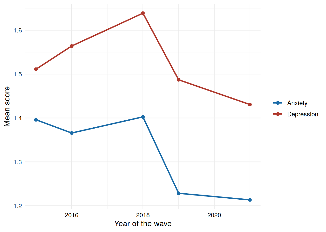
The variables are anx1 to anx5 and dep1 to dep5, measured at the same five waves, in 2015, 2016, 2018, 2019 and 2021. As in the earlier chapters, the time scores are 0, 1, 3, 4 and 6, with 2015 as time 0 and one unit equal to one year. The intercept factors therefore refer to the first wave and the slope factors to the change per year (see Chapter 1 and Biesanz et al. (2004) for why the coding of time matters).
Code
wave_means <-data.frame(year =rep(c(2015, 2016, 2018, 2019, 2021), 2),domain =rep(c("Anxiety", "Depression"), each =5),mean =c(colMeans(data[, paste0("anx", 1:5)], na.rm =TRUE),colMeans(data[, paste0("dep", 1:5)], na.rm =TRUE)))ggplot(wave_means, aes(x = year, y = mean, color = domain, group = domain)) +geom_line(linewidth =1) +geom_point(size =2) +scale_color_manual(values =c("Anxiety"="#1b6ca8", "Depression"="#b03a2e")) +labs(x ="Year of the wave", y ="Mean score", color =NULL)
Figure 9.1: Observed means of the anxiety and depression scores at the five waves. Each mean uses all participants with an observed score at that wave.
A participant is used in the models only if all ten scores are observed. The dataset has 442 rows, 321 of them with complete data on all ten variables, and the number of observed scores per wave is between 390 and 413. The workshop script uses growth() with its default settings, so the models are fitted with listwise deletion and N = 321 in every model (see Chapter 1 for the missing data handling).
The scores are positively skewed, with skewness between 1.477 and 3.821 across the ten variables, and most scores are close to the lowest values. The caution about non-normality in Chapter 1 applies to the chi-square statistic and the fit indices below.
A last descriptive result prepares the third model. Table 9.1 shows the correlations between the anxiety scores (rows) and the depression scores (columns) in the 321 participants with complete data. The correlation of the two domains at the same wave is on the diagonal. These correlations are between .66 and .77, with a mean of .73. Correlations between an anxiety score at one wave and a depression score at another wave are smaller, with a mean of .34. Remember this pattern when the fit of the models is compared.
Code
knitr::kable(round(cross, 2))
Table 9.1: Correlations between the anxiety scores (rows) and the depression scores (columns), complete cases.
dep1
dep2
dep3
dep4
dep5
anx1
0.71
0.48
0.35
0.22
0.17
anx2
0.49
0.76
0.42
0.35
0.29
anx3
0.39
0.46
0.74
0.39
0.32
anx4
0.27
0.32
0.37
0.77
0.27
anx5
0.26
0.32
0.37
0.35
0.66
9.4 The formal model
Within each domain the growth process is the linear growth model of Chapter 2. For participant \(i\) at wave \(t\), with time scores \(\lambda_t = (0, 1, 3, 4, 6)\),
The four growth factors ia (intercept of anxiety), sa (slope of anxiety), id (intercept of depression) and sd (slope of depression) have a mean vector \(\boldsymbol{\alpha}\) and a covariance matrix \(\boldsymbol{\Psi}\). The covariance matrix of the ten observed variables that the model implies is
where \(\boldsymbol{\Lambda}\) holds the fixed loadings (1 for the intercepts, the time scores for the slopes) and \(\boldsymbol{\Theta}\) is the covariance matrix of the residuals \(\epsilon_{ti}\) and \(\delta_{ti}\).
In the parallel growth model \(\boldsymbol{\Theta}\) is diagonal. Each residual has its own variance and no covariances. In the model with autocorrelated residuals, the covariance between \(\epsilon_{t}\) and \(\epsilon_{t+1}\) is set equal to a single parameter \(\theta_a\) for the four pairs of adjacent waves, and the covariance between \(\delta_{t}\) and \(\delta_{t+1}\) is set equal to \(\theta_d\). In the model with cross-domain residual covariances, the covariance between \(\epsilon_t\) and \(\delta_t\) is set equal to a single parameter \(\theta_{ad}\) at all five waves. The growth part is identical in the three models.
The model has 10 observed means and 55 observed variances and covariances, so there are 65 pieces of information. The parallel growth model estimates 22 parameters (4 growth factor means, 4 growth factor variances, 4 covariances among growth factors and 10 residual variances), which leaves 43 degrees of freedom. The two other models add parameters to this one.
9.5 The parallel growth model
9.5.1 R implementation
The first four lines define the two growth processes, with the same time scores that we used before. The lines below them concern the covariances among the growth factors. In the workshop script this is model 10.1.
lavaan 0.6.17 ended normally after 90 iterations

  Estimator                                         ML
  Optimization method                           NLMINB
  Number of model parameters                        22

                                                  Used       Total
  Number of observations                           321         442

Model Test User Model:

  Test statistic                               820.887
  Degrees of freedom                                43
  P-value (Chi-square)                           0.000

Model Test Baseline Model:

  Test statistic                              1912.994
  Degrees of freedom                                45
  P-value                                        0.000

User Model versus Baseline Model:

  Comparative Fit Index (CFI)                    0.584
  Tucker-Lewis Index (TLI)                       0.564

Loglikelihood and Information Criteria:

  Loglikelihood user model (H0)              -1711.078
  Loglikelihood unrestricted model (H1)      -1300.634

  Akaike (AIC)                                3466.156
  Bayesian (BIC)                              3549.128
  Sample-size adjusted Bayesian (SABIC)       3479.347

Root Mean Square Error of Approximation:

  RMSEA                                          0.237
  90 Percent confidence interval - lower         0.223
  90 Percent confidence interval - upper         0.252
  P-value H_0: RMSEA <= 0.050                    0.000
  P-value H_0: RMSEA >= 0.080                    1.000

Standardized Root Mean Square Residual:

  SRMR                                           0.357

Parameter Estimates:

  Standard errors                             Standard
  Information                                 Expected
  Information saturated (h1) model          Structured

Latent Variables:
                   Estimate  Std.Err  z-value  P(>|z|)
  ia =~
    anx1              1.000
    anx2              1.000
    anx3              1.000
    anx4              1.000
    anx5              1.000
  sa =~
    anx1              0.000
    anx2              1.000
    anx3              3.000
    anx4              4.000
    anx5              6.000
  id =~
    dep1              1.000
    dep2              1.000
    dep3              1.000
    dep4              1.000
    dep5              1.000
  sd =~
    dep1              0.000
    dep2              1.000
    dep3              3.000
    dep4              4.000
    dep5              6.000

Covariances:
                   Estimate  Std.Err  z-value  P(>|z|)
  ia ~~
    id                0.125    0.012   10.436    0.000
    sa                0.000    0.002    0.109    0.913
  id ~~
    sd                0.005    0.002    2.216    0.027
  sa ~~
    sd                0.004    0.000    9.146    0.000
  ia ~~
    sd                0.000
  sa ~~
    id                0.000

Intercepts:
                   Estimate  Std.Err  z-value  P(>|z|)
    ia                1.397    0.022   64.889    0.000
    sa               -0.032    0.004   -7.842    0.000
    id                1.545    0.027   56.861    0.000
    sd               -0.014    0.005   -2.825    0.005

Variances:
                   Estimate  Std.Err  z-value  P(>|z|)
   .anx1              0.083    0.010    8.647    0.000
   .anx2              0.122    0.011   11.095    0.000
   .anx3              0.148    0.012   11.878    0.000
   .anx4              0.103    0.009   11.541    0.000
   .anx5              0.062    0.008    7.615    0.000
   .dep1              0.103    0.012    8.309    0.000
   .dep2              0.149    0.014   10.787    0.000
   .dep3              0.241    0.020   11.889    0.000
   .dep4              0.181    0.016   11.601    0.000
   .dep5              0.156    0.017    9.292    0.000
    ia                0.097    0.012    8.393    0.000
    sa                0.002    0.000    3.997    0.000
    id                0.171    0.019    8.956    0.000
    sd                0.002    0.001    2.954    0.003
With growth(), lavaan lets all the growth factors covary by default. There are six possible covariances among four growth factors. The lines ia ~~ id + sa and sd ~~ id + sa ask for four of them: the covariance of the two intercept factors, the covariance of the two slope factors, and the covariance of intercept factor and slope factor within each domain. The two remaining covariances, between the anxiety intercept factor and the depression slope factor (ia ~~ 0*sd) and between the depression intercept factor and the anxiety slope factor (id ~~ 0*sa), are fixed to zero.
These two constraints are in the workshop code because the path diagram of the model (Figure 9.2) draws only four curved arrows between the growth factors. These are the two arrows within a domain (intercept factor with slope factor) and the two arrows between growth factors of the same kind (intercept factor with intercept factor and slope factor with slope factor). Fixing the other two covariances to zero makes the model equal to the diagram. The constraints are an assumption of the model. They state that the initial level of one domain is unrelated to the rate of change in the other domain. The workshop code does not test this assumption.
Figure 9.2: Path diagram of the parallel growth model. The upper part is the growth model for anxiety, the lower part is the growth model for depression. Look at the double-headed arrows between the two parts. They connect the two intercepts and the two slopes, and they carry the non-directional association between the two processes. Source: workshop slides (Anyan, 2023).
9.5.2 Understanding the output
The model converges and uses 321 of the 442 rows. Figure 9.3 shows the workshop slide with the results. The slide reports Mplus estimates. The numbers in this chapter are from the R output above, and they agree with the slide to the reported precision.
Figure 9.3: Results of the parallel growth model with the path diagram. Look at the fit statistics at the top and at the covariances at the bottom. Mplus estimates, as reported in the workshop. The depression intercept-slope covariance has no asterisk on the slide, whereas the R output gives p = .027. Source: workshop slides (Anyan, 2023).
The fit is poor. We find \(\chi^2(43) = 820.887\), CFI = .584, TLI = .564, RMSEA = .237 (90% CI .223 to .252) and SRMR = .357. These values are far from the usual reference values for an acceptable fit (Hu & Bentler, 1999). The model reproduces the covariances among the ten variables badly.
The anxiety intercept is 1.397 and the anxiety slope is -0.032 (p < .001). The depression intercept is 1.545 and the depression slope is -0.014 (p = .005). So the average level at the first wave is about 1.4 for anxiety and 1.5 for depression, and both averages decrease slightly per year. Over the six years from the first to the fifth wave, the model implies an average change of -0.192 for anxiety and -0.086 for depression, on the scale of the scores.
The variances of the growth factors are all different from zero according to the z tests. The variance of the intercept is 0.097 for anxiety and 0.171 for depression. The variance of the slope is only 0.002 for anxiety and 0.002 for depression. The slope variances are small in absolute terms, which is expected for a change per year.
The covariances among the growth factors answer the questions of the chapter, but the lavaan warning below must be kept in mind. It shows that the covariance of the two slopes cannot be interpreted. The covariance between the two intercepts is 0.125 (SE = 0.012, z = 10.436, p < .001). The covariance between the two slopes is 0.004 (z = 9.146, p < .001). Within the anxiety domain the covariance of intercept and slope is 0.000 (p = .913), and within the depression domain it is 0.005 (p = .027). The covariance of the two intercepts is positive, which means that participants who start higher on anxiety also start higher on depression.
9.5.3 The lavaan warning
lavaan prints a warning for this model: the covariance matrix of the latent variables is not positive definite. This is the covariance matrix of the four growth factors. A covariance matrix is not positive definite when some combination of the variables has a negative variance, which cannot happen for real variables. The estimates are then not a possible set of variances and covariances.
Table 9.2 collects the checks for the three models. For the parallel growth model, the variances of the four growth factors are positive, but the correlation between the two slopes that the estimates imply is 1.73. A correlation cannot be larger than 1. The covariance of the two slopes (0.0037) is larger than the product of the standard deviations of the slopes allows. The correlation between the two intercepts is .97, which is close to the limit. The smallest eigenvalue of the covariance matrix of the growth factors is -0.00237, and it is negative, which is how lavaan detects the problem.
Notice that each slope has a variance close to zero, and that a covariance with a factor that hardly varies is difficult to estimate. The slope covariance in this model is large relative to these variances. Therefore the covariance of the two slopes in this model is not a result that we can interpret.
9.6 The model with autocorrelated residuals
9.6.1 Why we add autocorrelations
The poor fit of the parallel growth model suggests that the residuals are not unrelated. A first candidate is the relation of a variable with itself over adjacent waves. After removing the person-specific line, a participant who scores above the line at one wave could still score above the line at the next wave. This is called an autocorrelated residual. The workshop slides draw these covariances as curved arrows between neighboring variables of a domain (Figure 9.4). The model does not say what the source of such a covariance is.
9.6.2 R implementation
In the workshop script this is model 10.2. Eight lines are added to the parallel growth model. The four lines for anxiety share the label eqa and the four lines for depression share the label eqd. Lines that share a label are held equal. Therefore the model has one autocorrelation for anxiety and one for depression, each assumed to be the same for all adjacent pairs of waves.
lavaan 0.6.17 ended normally after 117 iterations

  Estimator                                         ML
  Optimization method                           NLMINB
  Number of model parameters                        30
  Number of equality constraints                     6

                                                  Used       Total
  Number of observations                           321         442

Model Test User Model:

  Test statistic                               813.952
  Degrees of freedom                                41
  P-value (Chi-square)                           0.000

Model Test Baseline Model:

  Test statistic                              1912.994
  Degrees of freedom                                45
  P-value                                        0.000

User Model versus Baseline Model:

  Comparative Fit Index (CFI)                    0.586
  Tucker-Lewis Index (TLI)                       0.546

Loglikelihood and Information Criteria:

  Loglikelihood user model (H0)              -1707.610
  Loglikelihood unrestricted model (H1)      -1300.634

  Akaike (AIC)                                3463.221
  Bayesian (BIC)                              3553.735
  Sample-size adjusted Bayesian (SABIC)       3477.611

Root Mean Square Error of Approximation:

  RMSEA                                          0.242
  90 Percent confidence interval - lower         0.228
  90 Percent confidence interval - upper         0.257
  P-value H_0: RMSEA <= 0.050                    0.000
  P-value H_0: RMSEA >= 0.080                    1.000

Standardized Root Mean Square Residual:

  SRMR                                           0.352

Parameter Estimates:

  Standard errors                             Standard
  Information                                 Expected
  Information saturated (h1) model          Structured

Latent Variables:
                   Estimate  Std.Err  z-value  P(>|z|)
  ia =~
    anx1              1.000
    anx2              1.000
    anx3              1.000
    anx4              1.000
    anx5              1.000
  sa =~
    anx1              0.000
    anx2              1.000
    anx3              3.000
    anx4              4.000
    anx5              6.000
  id =~
    dep1              1.000
    dep2              1.000
    dep3              1.000
    dep4              1.000
    dep5              1.000
  sd =~
    dep1              0.000
    dep2              1.000
    dep3              3.000
    dep4              4.000
    dep5              6.000

Covariances:
                   Estimate  Std.Err  z-value  P(>|z|)
  ia ~~
    id                0.124    0.012   10.425    0.000
    sa                0.003    0.002    1.479    0.139
  id ~~
    sd                0.007    0.003    2.471    0.013
  sa ~~
    sd                0.004    0.000    9.102    0.000
  ia ~~
    sd                0.000
  sa ~~
    id                0.000
 .anx1 ~~
   .anx2     (eqa)    0.012    0.005    2.332    0.020
 .anx2 ~~
   .anx3     (eqa)    0.012    0.005    2.332    0.020
 .anx3 ~~
   .anx4     (eqa)    0.012    0.005    2.332    0.020
 .anx4 ~~
   .anx5     (eqa)    0.012    0.005    2.332    0.020
 .dep1 ~~
   .dep2     (eqd)    0.013    0.009    1.524    0.127
 .dep2 ~~
   .dep3     (eqd)    0.013    0.009    1.524    0.127
 .dep3 ~~
   .dep4     (eqd)    0.013    0.009    1.524    0.127
 .dep4 ~~
   .dep5     (eqd)    0.013    0.009    1.524    0.127

Intercepts:
                   Estimate  Std.Err  z-value  P(>|z|)
    ia                1.395    0.021   65.031    0.000
    sa               -0.031    0.004   -7.646    0.000
    id                1.544    0.027   56.969    0.000
    sd               -0.014    0.005   -2.738    0.006

Variances:
                   Estimate  Std.Err  z-value  P(>|z|)
   .anx1              0.096    0.011    8.413    0.000
   .anx2              0.131    0.012   11.072    0.000
   .anx3              0.154    0.013   11.825    0.000
   .anx4              0.112    0.010   11.487    0.000
   .anx5              0.078    0.011    6.809    0.000
   .dep1              0.114    0.016    7.271    0.000
   .dep2              0.160    0.016   10.137    0.000
   .dep3              0.245    0.021   11.736    0.000
   .dep4              0.192    0.017   11.539    0.000
   .dep5              0.173    0.022    7.970    0.000
    ia                0.084    0.013    6.470    0.000
    sa                0.001    0.001    1.519    0.129
    id                0.156    0.021    7.327    0.000
    sd                0.001    0.001    1.201    0.230
The equality constraint is a simplification. The waves are one, two, one and two years apart, and the dependence between residuals of waves that are two years apart need not be the same as for waves that are one year apart. Holding the covariances equal keeps the model small.
Figure 9.4: Path diagram of the model with autocorrelated residuals. Look at the green curved arrows between neighboring observed variables within each domain. They are the residual covariances that are added to the parallel growth model. Source: workshop slides (Anyan, 2023).
9.6.3 Understanding the output
Figure 9.5 shows the slide with the results. It reports Mplus estimates, and the lower part of the slide is cropped. The chapter uses the R output.
Figure 9.5: Results of the model with autocorrelated residuals. Look at the fit statistics, which are almost the same as in the parallel growth model, and at the autocorrelation of anxiety at the bottom. Mplus estimates, as reported in the workshop. Source: workshop slides (Anyan, 2023).
The model uses the same 321 participants. The fit is as poor as before: \(\chi^2(41) = 813.952\), CFI = .586, TLI = .546, RMSEA = .242 (90% CI .228 to .257) and SRMR = .352. The model has two more parameters than the parallel growth model, so two degrees of freedom less.
The autocorrelation for anxiety (eqa) is 0.012 (SE = 0.005, z = 2.332, p = .020). The autocorrelation for depression (eqd) is 0.013 (SE = 0.009, z = 1.524, p = .127). The two values are similar in size, but only the first is distinguishable from zero given its standard error. On the correlation scale, the residuals of adjacent waves correlate about .11 for anxiety and .10 for depression. These are small correlations.
The growth factors change as well. The slope variances are 0.001 for anxiety (p = .129) and 0.001 for depression (p = .230). In the parallel growth model both slope variances were significant. Now neither is distinguishable from zero. Some of the variation that was assigned to the slopes in the parallel growth model may be wave-specific variation that is now taken by the residual covariances.
The same warning appears again. The covariance matrix of the latent variables is not positive definite. The variances of the slopes are positive, but the estimated covariance between the two slopes (0.004) implies a correlation of 3.20, and the correlation of the two intercepts is 1.09. Both are above 1 (see Table 9.2).
9.6.4 What changed compared with the parallel growth model
The parallel growth model is the model with autocorrelated residuals in which the two autocorrelations are fixed at zero. So the two models are nested, and the likelihood ratio test applies. The change in fit is small. The chi-square decreases by 6.935 for two degrees of freedom. This suggests that carryover from wave to wave within a domain is a small part of what the first model misses.
9.7 The model with cross-domain residual covariances
9.7.1 Why we add cross-domain covariances
The correlations in Table 9.1 suggest another place to look. The two domains correlate strongly at the same wave and much less across different waves. The growth factors describe differences between persons that are stable over the waves. Because the slope variances are small, they mainly imply a covariance between an anxiety score and a depression score that is similar for any pair of waves. The data show a much higher covariance at the same wave. This is a covariance between the residuals of the two domains, specific to the wave. The workshop slides label it the time-specific component between the domains (Figure 9.6).
9.7.2 R implementation
In the workshop script this is model 10.3. The five new lines connect the anxiety residual with the depression residual at the same wave, and they all share the label eq. The autocorrelations of the previous model are not part of this model.
lavaan 0.6.17 ended normally after 106 iterations

  Estimator                                         ML
  Optimization method                           NLMINB
  Number of model parameters                        27
  Number of equality constraints                     4

                                                  Used       Total
  Number of observations                           321         442

Model Test User Model:

  Test statistic                               178.746
  Degrees of freedom                                42
  P-value (Chi-square)                           0.000

Model Test Baseline Model:

  Test statistic                              1912.994
  Degrees of freedom                                45
  P-value                                        0.000

User Model versus Baseline Model:

  Comparative Fit Index (CFI)                    0.927
  Tucker-Lewis Index (TLI)                       0.922

Loglikelihood and Information Criteria:

  Loglikelihood user model (H0)              -1390.007
  Loglikelihood unrestricted model (H1)      -1300.634

  Akaike (AIC)                                2826.015
  Bayesian (BIC)                              2912.758
  Sample-size adjusted Bayesian (SABIC)       2839.805

Root Mean Square Error of Approximation:

  RMSEA                                          0.101
  90 Percent confidence interval - lower         0.086
  90 Percent confidence interval - upper         0.116
  P-value H_0: RMSEA <= 0.050                    0.000
  P-value H_0: RMSEA >= 0.080                    0.988

Standardized Root Mean Square Residual:

  SRMR                                           0.141

Parameter Estimates:

  Standard errors                             Standard
  Information                                 Expected
  Information saturated (h1) model          Structured

Latent Variables:
                   Estimate  Std.Err  z-value  P(>|z|)
  ia =~
    anx1              1.000
    anx2              1.000
    anx3              1.000
    anx4              1.000
    anx5              1.000
  sa =~
    anx1              0.000
    anx2              1.000
    anx3              3.000
    anx4              4.000
    anx5              6.000
  id =~
    dep1              1.000
    dep2              1.000
    dep3              1.000
    dep4              1.000
    dep5              1.000
  sd =~
    dep1              0.000
    dep2              1.000
    dep3              3.000
    dep4              4.000
    dep5              6.000

Covariances:
                   Estimate  Std.Err  z-value  P(>|z|)
  ia ~~
    id                0.082    0.009    8.799    0.000
    sa               -0.004    0.001   -2.758    0.006
  id ~~
    sd               -0.002    0.002   -0.821    0.412
  sa ~~
    sd               -0.000    0.000   -0.550    0.583
  ia ~~
    sd                0.000
  sa ~~
    id                0.000
 .anx1 ~~
   .dep1      (eq)    0.098    0.005   18.539    0.000
 .anx2 ~~
   .dep2      (eq)    0.098    0.005   18.539    0.000
 .anx3 ~~
   .dep3      (eq)    0.098    0.005   18.539    0.000
 .anx4 ~~
   .dep4      (eq)    0.098    0.005   18.539    0.000
 .anx5 ~~
   .dep5      (eq)    0.098    0.005   18.539    0.000

Intercepts:
                   Estimate  Std.Err  z-value  P(>|z|)
    ia                1.399    0.022   64.538    0.000
    sa               -0.030    0.004   -7.489    0.000
    id                1.552    0.027   57.861    0.000
    sd               -0.013    0.005   -2.567    0.010

Variances:
                   Estimate  Std.Err  z-value  P(>|z|)
   .anx1              0.121    0.009   13.276    0.000
   .anx2              0.130    0.009   14.738    0.000
   .anx3              0.129    0.009   14.955    0.000
   .anx4              0.103    0.007   15.580    0.000
   .anx5              0.083    0.007   11.318    0.000
   .dep1              0.152    0.012   12.969    0.000
   .dep2              0.164    0.011   14.507    0.000
   .dep3              0.205    0.014   14.791    0.000
   .dep4              0.180    0.012   15.351    0.000
   .dep5              0.215    0.015   13.862    0.000
    ia                0.085    0.010    8.608    0.000
    sa                0.001    0.000    2.106    0.035
    id                0.144    0.016    8.928    0.000
    sd               -0.000    0.001   -0.214    0.831
Figure 9.6: Path diagram of the model with cross-domain residual covariances. Look at the green curved arrows between the anxiety and the depression variable of the same wave. They are the residual covariances that are added to the parallel growth model. Source: workshop slides (Anyan, 2023).
9.7.3 Understanding the output
Figure 9.7 shows the workshop slide with the results. It reports Mplus estimates, and the lower part of the slide is cropped, but the cross-domain covariance is visible. The chapter uses the R output.
Figure 9.7: Results of the model with cross-domain residual covariances. Look at the fit statistics, which are much better than in the two previous models, and at the covariances among the growth factors, which have changed. Mplus estimates, as reported in the workshop. The slide reports 0.000 for the variance of the depression slope. Source: workshop slides (Anyan, 2023).
The model again uses 321 participants and has one parameter more than the parallel growth model. The fit improves a great deal: \(\chi^2(42) = 178.746\), CFI = .927, TLI = .922, RMSEA = .101 (90% CI .086 to .116) and SRMR = .141. This is the best fit of the three models, but it is not a well fitting model by the usual reference values (Hu & Bentler, 1999). The CFI is below .95, and the RMSEA and the SRMR are above .08. The substantive reading below is therefore tentative.
The cross-domain residual covariance (eq) is 0.098 (SE = 0.005, z = 18.539, p < .001). On the correlation scale this is .72 at the first wave and .73 at the fifth wave. This is a large amount of shared wave-specific variation. After removing the growth factors, the anxiety and the depression scores of the same wave still correlate between .60 and .73 across the five waves.
The covariance is held equal across waves, but the residual variances differ between waves, so the standardized correlation differs too (.60 at the third wave, against .72 and .73 at the first and the fifth). The equality constraint has not been tested here.
The growth factors change as well.
The covariance of the two intercepts decreases from 0.125 to 0.082, and it remains clearly positive (SE = 0.009, z = 8.799, p < .001). The correlation of the intercepts falls from .97 in the parallel growth model to about .75.
The covariance of the two slopes is -0.0002 (p = .583). In the two previous models it was 0.004 (p < .001) and 0.004 (p < .001). It involves the depression slope factor, whose variance is negative in this model, and it cannot be interpreted (see the warning below).
The covariance of intercept and slope in anxiety is now -0.004 (p = .006). In depression it is -0.002 (p = .412).
The average growth factors hardly change. The anxiety intercept and slope are 1.399 and -0.030. The depression intercept and slope are 1.552 and -0.013.
9.7.4 The lavaan warning
For this model lavaan warns that some estimated latent variances are negative. The negative variance is that of the depression slope factor (sd). Its estimate is -0.0001 (SE = 0.0006, z = -0.214, p = .831). Negative variance estimates of this kind are discussed by Dillon et al. (1987). A variance cannot be negative, so the estimate has to be read as zero. The standard error is larger than the estimate, which means that the data are consistent with a variance of exactly zero. In this model, once the shared wave-specific variation has been taken out, there is no detectable variation between persons in the rate of change in depression. In the parallel growth model the variance of the depression slope is 0.002 (p = .003), so the result depends on the model. The variance of the slope of anxiety is also small (0.001, p = .035).
This has consequences for the covariances of the depression slope. A correlation with a factor that has no variance is not defined. For this reason Table 9.2 cannot report the correlation of the depression slope factor with the other growth factors for this model, and the covariances of sd in the output (with id and with sa) should not be interpreted.
Table 9.2: Checks on the covariance matrix of the four growth factors in the three models. The correlations are computed from the estimated variances and covariances. A correlation is missing when a variance is negative.
Variance sa
Variance sd
Smallest eigenvalue
Correlation ia, id
Correlation sa, sd
Parallel growth model
0.0019
0.0023
-0.0024
0.9700
1.7315
Autocorrelated residuals
0.0010
0.0013
-0.0119
1.0864
3.2015
Cross-domain residual covariances
0.0009
-0.0001
-0.0002
0.7451
not defined
A covariance can be significant and still be impossible
In the parallel growth model and in the model with autocorrelated residuals the covariance of the two slopes has a very small standard error, and it looks like the most precisely estimated result of the model. Table 9.2 shows that it corresponds to a correlation above 1. This is not possible. The estimates reach this value because the slope variances are close to zero while the covariance is not. Check the implied correlations with cov2cor(lavInspect(fit, "cov.lv")) whenever lavaan reports a latent covariance matrix that is not positive definite, before interpreting covariances among growth factors.
In such a case a researcher can fix the variance of the slope factor to zero, drop the slope factor of that domain, or use more data. We do not change the workshop syntax here.
9.7.5 What changed compared with the previous models
The only change from the parallel growth model is the five residual covariances held equal, which is one parameter. The change in fit is large, and it is a statement about the correspondence between the model and the data. The data contain a large covariance between the two domains at the same wave, and the first two models had no way to represent it. The growth factors may have absorbed it, which may be why the intercepts correlated almost perfectly and why the slope covariance was an impossible value. When the same-wave covariance is allowed, the growth factors take more modest values.
9.8 Comparing the three models
Table 9.3 puts the fit of the three models next to each other.
Table 9.3: Fit of the three models, N = 321 (listwise deletion). AIC and BIC are smaller for models that fit better.
Chi-square
df
CFI
RMSEA
SRMR
AIC
BIC
Parallel growth model
820.887
43
0.584
0.237
0.357
3466.156
3549.128
Autocorrelated residuals
813.952
41
0.586
0.242
0.352
3463.221
3553.735
Cross-domain residual covariances
178.746
42
0.927
0.101
0.141
2826.015
2912.758
The first two models are nested. The parallel growth model results from the model with autocorrelated residuals when eqa and eqd are fixed at zero. The chi-square difference test of the two (Bentler & Bonett, 1980) is
The reduced model is rejected at the .05 level, so the model with the two autocorrelations fits better in the statistical sense. The difference is small, 6.935 for two degrees of freedom, and both models fit very poorly. The Akaike information criterion (AIC, Akaike, 1974) prefers the model with autocorrelated residuals (3463.221 against 3466.156), and the Bayesian information criterion (BIC, Schwarz, 1978) prefers the parallel growth model (3549.128 against 3553.735). Remember that models should be compared in substantive terms only if their fit is acceptable. A statistically significant difference between two models that both fit badly does not make the better one a good model. Also, the usual reference distribution of the test does not hold when a variance is estimated at or near the boundary of zero (Self & Liang, 1987), which is the case here (see the warnings above), so the p value is approximate.
Nested and non-nested models
The parallel growth model is nested in each of the two other models, because it is obtained by fixing their added parameters at zero. So anova(fit_parallel, fit_parallelcross) is a valid likelihood ratio test, with a chi-square difference of 642.141 for one degree of freedom. The model with autocorrelated residuals and the model with cross-domain residual covariances are not nested, because each has parameters that the other does not have. Their chi-square values cannot be tested against each other. Information criteria can be compared for non-nested models fitted to the same data, which is the case here.
The model with cross-domain residual covariances has an AIC of 2826.015 and a BIC of 2912.758. Both are lower than the values of the model with autocorrelated residuals, by 637.206 (AIC) and 640.978 (BIC), and this agrees with all fit indices in Table 9.3. The comparison with the second model is made with the information criteria alone. Both criteria and all fit indices put the model with cross-domain residual covariances first. The order of the two other models depends on the criterion.
9.9 Sensitivity to the missing data handling
The models above are based on 321 of the 442 rows. As a check, which is not part of the workshop, the three models were also fitted with full information maximum likelihood (FIML, see Chapter 1). FIML was found to perform better than listwise deletion in the conditions examined by Enders & Bandalos (2001).
Table 9.4: Sensitivity analysis, not part of the workshop. Fit of the three models with listwise deletion and with FIML.
Model
N_listwise
CFI
RMSEA
N_FIML
CFI_FIML
RMSEA_FIML
SRMR_FIML
Parallel growth model
321
0.584
0.237
436
0.625
0.223
0.356
Autocorrelated residuals
321
0.586
0.242
436
0.628
0.228
0.350
Cross-domain residual covariances
321
0.927
0.101
436
0.942
0.089
0.127
The FIML models use N = 436. The pattern is the same as with listwise deletion. The first two models fit poorly (CFI .625 and .628), and the model with cross-domain residual covariances fits better (CFI .942, RMSEA .089, SRMR .127). With the robust maximum likelihood estimator (Yuan & Bentler, 2000) and FIML, the CFI of the third model is .954, which meets the usual cut-off of .95, and the RMSEA is .083. The RMSEA and the SRMR under FIML are still above .08 (Hu & Bentler, 1999).
The growth factor means hardly change. For example, the anxiety intercept in the model with cross-domain residual covariances is 1.399 with listwise deletion and 1.413 with FIML. The variances are somewhat larger under FIML, for instance the variance of the anxiety intercept in this model is 0.085 and 0.106. The cross-domain residual covariance is 0.098 and 0.103. The variance of the depression slope in this model is 0.00028 under FIML (SE = 0.00065) against -0.00014 with listwise deletion. Under FIML the estimate is positive, but it is not distinguishable from zero. So the factor has little variance to estimate in both analyses.
The correlation of the two intercepts is 1.00 in the parallel growth model and .77 in the model with cross-domain residual covariances under FIML. This is the same pattern as with listwise deletion, with a value at or just above the limit of 1 in the first model.
9.10 A check on the two constraints at zero
The two covariances that are fixed at zero, ia ~~ 0*sd and id ~~ 0*sa, are part of the three workshop models. Nothing in the data requires them, so we can check what happens when they are estimated. The code below is an addition to the workshop. It is the model with cross-domain residual covariances, with the two covariances freed.
Code
# Addition, not part of the workshop: the two covariances fixed at zero are freedparallelcross_free <-' ia =~ 1*anx1 + 1*anx2 + 1*anx3 + 1*anx4 + 1*anx5 sa =~ 0*anx1 + 1*anx2 + 3*anx3 + 4*anx4 + 6*anx5 id =~ 1*dep1 + 1*dep2 + 1*dep3 + 1*dep4 + 1*dep5 sd =~ 0*dep1 + 1*dep2 + 3*dep3 + 4*dep4 + 6*dep5ia ~~ id + sa + sdsd ~~ id + said ~~ saanx1 ~~ eq*dep1anx2 ~~ eq*dep2anx3 ~~ eq*dep3anx4 ~~ eq*dep4anx5 ~~ eq*dep5'fit_parallelcross_free <-growth(parallelcross_free, data = data)anova(fit_parallelcross, fit_parallelcross_free)
parameterEstimates(fit_parallelcross_free) |>filter(op =="~~", lhs %in%c("ia", "sa", "id", "sd"), rhs %in%c("ia", "sa", "id", "sd")) |>select(lhs, rhs, est, se, z, pvalue)
   lhs rhs    est    se      z pvalue
1   ia  id  0.127 0.016  7.903  0.000
2   ia  sa -0.011 0.002 -4.487  0.000
3   ia  sd -0.009 0.003 -3.575  0.000
4   id  sd -0.012 0.003 -3.488  0.000
5   sa  sd  0.001 0.001  2.649  0.008
6   sa  id -0.010 0.003 -3.690  0.000
7   ia  ia  0.120 0.015  8.125  0.000
8   sa  sa  0.002 0.001  3.817  0.000
9   id  id  0.191 0.022  8.657  0.000
10  sd  sd  0.002 0.001  2.045  0.041
lavaan gives no warning for this model, and all four growth factor variances are positive. The smallest eigenvalue of the covariance matrix of the growth factors is 0.00027, so the matrix is positive definite. The model fits better than the model of the workshop: \(\chi^2(40) = 158.729\), CFI = .936, RMSEA = .096 and SRMR = .121. The chi-square difference with the model of the workshop (Bentler & Bonett, 1980) is 20.017 for two degrees of freedom. The two freed covariances are -0.009 (anxiety intercept with depression slope) and -0.010 (depression intercept with anxiety slope), and the output shows that both are distinguishable from zero.
So the two constraints at zero are not harmless in this dataset. They may be part of the reason why a negative slope variance appears in the model with cross-domain residual covariances. We should not make much of the particular values of these covariances. They involve slope factors with variances of 0.002 and 0.002 (p = .041 for the depression slope factor, which is positive here), and such correlations are unstable. The fit, even with the covariances freed, is still not good by the usual reference values. Thus, a warning about a latent variance can come from a constraint we imposed.
9.11 What these models answer and what they cannot tell
The parallel growth model answers the question whether two growth processes are associated across persons. In this dataset the initial levels of anxiety and depression are positively related in all three models, and the association is strong. The correlation of the intercepts is .97 and 1.09 in the first two models (the second is above 1) and about .75 in the model with cross-domain residual covariances, which fits best of the three but is still not a well fitting model. The association between the two rates of change cannot be read from these models. In the first two it corresponds to a correlation above 1, and in the third the depression slope factor has a negative variance. With the two covariances freed the implied correlation of the slopes is .78, but the slope variances are very small, so this value is unstable. The data do not allow a strong claim about the co-development of the rates of change.
The models do not tell why the two domains covary at the same wave. The covariance of the residuals in the third model absorbs everything that is shared by the anxiety and the depression score of a wave and is not carried by the growth factors. The data do not tell us what this shared variation is. The models also do not give a direction. A parallel growth model does not describe an influence of one process on the other, and both processes cover the same period. A model in which one process comes before the other in time is the topic of Chapter 10.
9.12 Researcher’s perspective
The models use 321 of 442 rows. A model with two outcomes needs complete data on both, so the loss of cases is larger than in a single-outcome model. Report the N used, and consider FIML as a check.
Residual covariances can change the growth factors considerably, as the change of the slope variances and of the slope covariance shows. Models that differ only in the residual structure can give different answers to the same question about the growth factors. It is therefore useful to report more than one structure when the choice is not clear, and to say which one is used for the substantive reading.
The autocorrelations are held equal across waves that are one and two years apart, and the cross-domain covariance is held equal across five waves. These constraints are common, and they can be relaxed and tested if the sample is large enough. The constraints at zero between the growth factors of different domains define the model in the workshop, and they can be freed.
What to report
Report the N used and the method for missing data, the fit indices of each model including those that fit badly, any lavaan warning and what it refers to, the implied correlations among the growth factors if a warning about the latent covariance matrix appears, and which residual structure the substantive reading is based on. State that the improvement in fit from the residual covariances is a statement about how well the model reproduces the data.
Akaike, H. (1974). A new look at the statistical model identification. IEEE Transactions on Automatic Control, 19(6), 716–723. https://doi.org/10.1109/TAC.1974.1100705
Anyan, F. (2023). Longitudinal data analysis using Mplus and R. Workshop slides.
Bentler, P. M., & Bonett, D. G. (1980). Significance tests and goodness of fit in the analysis of covariance structures. Psychological Bulletin, 88(3), 588–606. https://doi.org/10.1037/0033-2909.88.3.588
Biesanz, J. C., Deeb-Sossa, N., Papadakis, A. A., Bollen, K. A., & Curran, P. J. (2004). The role of coding time in estimating and interpreting growth curve models. Psychological Methods, 9(1), 30–52. https://doi.org/10.1037/1082-989X.9.1.30
Bollen, K. A., & Curran, P. J. (2006). Latent curve models: A structural equation perspective. Wiley.
Cheong, J., MacKinnon, D. P., & Khoo, S. T. (2003). Investigation of mediational processes using parallel process latent growth curve modeling. Structural Equation Modeling: A Multidisciplinary Journal, 10(2), 238–262. https://doi.org/10.1207/S15328007SEM1002_5
Dillon, W. R., Kumar, A., & Mulani, N. (1987). Offending estimates in covariance structure analysis: Comments on the causes of and solutions to Heywood cases. Psychological Bulletin, 101(1), 126–135. https://doi.org/10.1037/0033-2909.101.1.126
Enders, C. K., & Bandalos, D. L. (2001). The relative performance of full information maximum likelihood estimation for missing data in structural equation models. Structural Equation Modeling: A Multidisciplinary Journal, 8(3), 430–457. https://doi.org/10.1207/S15328007SEM0803_5
Hu, L., & Bentler, P. M. (1999). Cutoff criteria for fit indexes in covariance structure analysis: Conventional criteria versus new alternatives. Structural Equation Modeling: A Multidisciplinary Journal, 6(1), 1–55. https://doi.org/10.1080/10705519909540118
Schwarz, G. (1978). Estimating the dimension of a model. The Annals of Statistics, 6(2), 461–464.
Self, S. G., & Liang, K.-Y. (1987). Asymptotic properties of maximum likelihood estimators and likelihood ratio tests under nonstandard conditions. Journal of the American Statistical Association, 82(398), 605–610. https://doi.org/10.1080/01621459.1987.10478472
Yuan, K.-H., & Bentler, P. M. (2000). Three likelihood-based methods for mean and covariance structure analysis with nonnormal missing data. Sociological Methodology, 30, 165–200.
Source Code
# Parallel process growth models {#sec-parallel}```{r}#| label: setup#| include: falselibrary(lavaan)library(dplyr)library(tidyr)library(ggplot2)library(psych)data <-read.csv("data/data.csv", fileEncoding ="UTF-8-BOM")theme_set(theme_minimal(base_size =12) +theme(plot.title =element_text(face ="bold", color ="black"),axis.title =element_text(color ="black"),axis.text =element_text(color ="black"),strip.text =element_text(color ="black"),legend.text =element_text(color ="black")))```In the previous chapters one process was followed at a time. The models of @sec-basic to @sec-multigroup described the growth of a single variable, loneliness, and asked what predicts it, what it predicts, or whether it differs between groups. Here, we follow two processes, anxiety symptoms and depression symptoms, in the same participants over the same five waves, and ask how the two growth processes relate to each other.A model that describes two or more growth processes at the same time is called a *parallel process growth model*, and parallel process latent growth models have been used to study the relations between growth processes [@cheong2003parallel]. The general treatment of latent curve models in the structural equation framework is in @bollen2006latent. The chapter fits three models. The first has covariances among the growth factors, the second adds covariances between the residuals of adjacent waves within each domain, and the third replaces these with covariances between the residuals of the two domains at the same wave. In the workshop script these are models 10.1, 10.2 and 10.3. We call them the *parallel growth model*, the *model with autocorrelated residuals* and the *model with cross-domain residual covariances*.## Why this modelA univariate growth model gives an initial level and a rate of change for one variable, and the variation of these between persons. It cannot say whether the persons who start high on one variable also start high on another, or whether the persons who change fastest on one variable also change fastest on another. For this we need both processes in one model, so that their growth factors can be correlated directly.The model can answer questions about how the two processes develop together.- Is the initial level of anxiety symptoms related to the initial level of depression symptoms?- Is the rate of change in anxiety symptoms related to the rate of change in depression symptoms?- How much of the association between the two domains is carried by the growth factors, and how much is left in the residuals at the individual waves?The associations in this model are non-directional. This is stated on the first slide of the model (@fig-parallel-diagram). The model describes two processes that occur together. It does not state that one process drives the other.## The idea in plain languageEach participant has an anxiety trajectory and a depression trajectory. Each trajectory is summarized in the way we summarized the trajectory of loneliness before, by an initial level and a rate of change. So every participant is described by four numbers: the initial level of anxiety, the rate of change in anxiety, the initial level of depression and the rate of change in depression. These four numbers are the growth factors, and they vary between persons.The parallel growth model is two linear growth models (see @sec-basic) fitted together. They are joined through the growth factors, which are allowed to covary. Whatever is left at each wave after removing the person-specific line is the residual of that wave. The three models of this chapter differ only in what we allow the residuals to do.In the parallel growth model the residuals are assumed to be unrelated to each other. In the model with autocorrelated residuals the residual of a variable at one wave is allowed to covary with the residual of the same variable at the next wave. In the model with cross-domain residual covariances the residual of anxiety at one wave is allowed to covary with the residual of depression at the same wave.## A concrete example with the datasetThe variables are `anx1` to `anx5` and `dep1` to `dep5`, measured at the same five waves, in 2015, 2016, 2018, 2019 and 2021. As in the earlier chapters, the time scores are 0, 1, 3, 4 and 6, with 2015 as time 0 and one unit equal to one year. The intercept factors therefore refer to the first wave and the slope factors to the change per year (see @sec-prelims and @biesanz2004coding for why the coding of time matters).```{r}#| label: fig-wave-means#| fig-cap: "Observed means of the anxiety and depression scores at the five waves. Each mean uses all participants with an observed score at that wave."#| fig-alt: "Line plot of the observed means of the anxiety and depression scores at the waves of 2015, 2016, 2018, 2019 and 2021."wave_means <-data.frame(year =rep(c(2015, 2016, 2018, 2019, 2021), 2),domain =rep(c("Anxiety", "Depression"), each =5),mean =c(colMeans(data[, paste0("anx", 1:5)], na.rm =TRUE),colMeans(data[, paste0("dep", 1:5)], na.rm =TRUE)))ggplot(wave_means, aes(x = year, y = mean, color = domain, group = domain)) +geom_line(linewidth =1) +geom_point(size =2) +scale_color_manual(values =c("Anxiety"="#1b6ca8", "Depression"="#b03a2e")) +labs(x ="Year of the wave", y ="Mean score", color =NULL)``````{r}#| label: helpers#| include: falseanx <-paste0("anx", 1:5)dep <-paste0("dep", 1:5)n_all <-nrow(data)n_cc <-sum(complete.cases(data[, c(anx, dep)]))n_wave <-colSums(!is.na(data[, c(anx, dep)]))r_obs <-cor(data[complete.cases(data[, c(anx, dep)]), c(anx, dep)])cross <- r_obs[anx, dep]r_same <-mean(diag(cross))r_diff <-mean(cross[row(cross) !=col(cross)])skw <-read.csv("data/diag/skew_kurtosis.csv")skw <- skw[skw$var %in%c(anx, dep), ]f3 <-function(x) sprintf("%.3f", x)f5 <-function(x) sprintf("%.5f", x)rl <-function(fit) suppressWarnings(cov2cor(lavInspect(fit, "cov.lv")))latent_check <-function(fit) { cv <-lavInspect(fit, "cov.lv") r <-rl(fit)c("Variance sa"= cv["sa", "sa"], "Variance sd"= cv["sd", "sd"],"Smallest eigenvalue"=min(eigen(cv)$values),"Correlation ia, id"= r["ia", "id"], "Correlation sa, sd"= r["sa", "sd"])}fx <-function(x, d =3) sub("^(-?)0\\.", "\\1.", sprintf(paste0("%.", d, "f"), x))pfmt <-function(p) ifelse(p < .001, "< .001", paste0("= ", fx(p)))getp <-function(fit, lhs, op, rhs) { p <-parameterEstimates(fit) p[p$lhs == lhs & p$op == op & p$rhs == rhs, ][1, ]}E <-function(fit, lhs, op, rhs, d =3) sprintf(paste0("%.", d, "f"), getp(fit, lhs, op, rhs)$est)SE <-function(fit, lhs, op, rhs, d =3) sprintf(paste0("%.", d, "f"), getp(fit, lhs, op, rhs)$se)ZV <-function(fit, lhs, op, rhs) sprintf("%.3f", getp(fit, lhs, op, rhs)$z)PV <-function(fit, lhs, op, rhs) pfmt(getp(fit, lhs, op, rhs)$pvalue)FM <-function(fit, m) fx(fitMeasures(fit, m))CH <-function(fit) sprintf("%.3f", fitMeasures(fit, "chisq"))```A participant is used in the models only if all ten scores are observed. The dataset has `r n_all` rows, `r n_cc` of them with complete data on all ten variables, and the number of observed scores per wave is between `r min(n_wave)` and `r max(n_wave)`. The workshop script uses `growth()` with its default settings, so the models are fitted with listwise deletion and N = `r n_cc` in every model (see @sec-prelims for the missing data handling).The scores are positively skewed, with skewness between `r f3(min(skw$skew))` and `r f3(max(skw$skew))` across the ten variables, and most scores are close to the lowest values. The caution about non-normality in @sec-prelims applies to the chi-square statistic and the fit indices below.A last descriptive result prepares the third model. @tbl-cross-cor shows the correlations between the anxiety scores (rows) and the depression scores (columns) in the `r n_cc` participants with complete data. The correlation of the two domains at the same wave is on the diagonal. These correlations are between `r fx(min(diag(cross)), 2)` and `r fx(max(diag(cross)), 2)`, with a mean of `r fx(r_same, 2)`. Correlations between an anxiety score at one wave and a depression score at another wave are smaller, with a mean of `r fx(r_diff, 2)`. Remember this pattern when the fit of the models is compared.```{r}#| label: tbl-cross-cor#| tbl-cap: "Correlations between the anxiety scores (rows) and the depression scores (columns), complete cases."knitr::kable(round(cross, 2))```## The formal modelWithin each domain the growth process is the linear growth model of @sec-basic. For participant $i$ at wave $t$, with time scores $\lambda_t = (0, 1, 3, 4, 6)$,$$\text{anx}_{ti} = \text{ia}_i + \lambda_t \, \text{sa}_i + \epsilon_{ti}, \qquad\text{dep}_{ti} = \text{id}_i + \lambda_t \, \text{sd}_i + \delta_{ti}.$$The four growth factors ia (intercept of anxiety), sa (slope of anxiety), id (intercept of depression) and sd (slope of depression) have a mean vector $\boldsymbol{\alpha}$ and a covariance matrix $\boldsymbol{\Psi}$. The covariance matrix of the ten observed variables that the model implies is$$\boldsymbol{\Sigma} = \boldsymbol{\Lambda} \boldsymbol{\Psi} \boldsymbol{\Lambda}' + \boldsymbol{\Theta},$$where $\boldsymbol{\Lambda}$ holds the fixed loadings (1 for the intercepts, the time scores for the slopes) and $\boldsymbol{\Theta}$ is the covariance matrix of the residuals $\epsilon_{ti}$ and $\delta_{ti}$.In the parallel growth model $\boldsymbol{\Theta}$ is diagonal. Each residual has its own variance and no covariances. In the model with autocorrelated residuals, the covariance between $\epsilon_{t}$ and $\epsilon_{t+1}$ is set equal to a single parameter $\theta_a$ for the four pairs of adjacent waves, and the covariance between $\delta_{t}$ and $\delta_{t+1}$ is set equal to $\theta_d$. In the model with cross-domain residual covariances, the covariance between $\epsilon_t$ and $\delta_t$ is set equal to a single parameter $\theta_{ad}$ at all five waves. The growth part is identical in the three models.The model has 10 observed means and 55 observed variances and covariances, so there are 65 pieces of information. The parallel growth model estimates 22 parameters (4 growth factor means, 4 growth factor variances, 4 covariances among growth factors and 10 residual variances), which leaves 43 degrees of freedom. The two other models add parameters to this one.## The parallel growth model### R implementationThe first four lines define the two growth processes, with the same time scores that we used before. The lines below them concern the covariances among the growth factors. In the workshop script this is model 10.1.```{r}#| label: parallel-modelparallel <-' ia =~ 1*anx1 + 1*anx2 + 1*anx3 + 1*anx4 + 1*anx5 sa =~ 0*anx1 + 1*anx2 + 3*anx3 + 4*anx4 + 6*anx5 id =~ 1*dep1 + 1*dep2 + 1*dep3 + 1*dep4 + 1*dep5 sd =~ 0*dep1 + 1*dep2 + 3*dep3 + 4*dep4 + 6*dep5#Growth factor corelationsia ~~ id + sasd ~~ id + saia ~~ 0*sdid ~~ 0*sa'fit_parallel <-growth(parallel, data = data)summary(fit_parallel, fit.measures =TRUE)```With `growth()`, lavaan lets all the growth factors covary by default. There are six possible covariances among four growth factors. The lines `ia ~~ id + sa` and `sd ~~ id + sa` ask for four of them: the covariance of the two intercept factors, the covariance of the two slope factors, and the covariance of intercept factor and slope factor within each domain. The two remaining covariances, between the anxiety intercept factor and the depression slope factor (`ia ~~ 0*sd`) and between the depression intercept factor and the anxiety slope factor (`id ~~ 0*sa`), are fixed to zero.These two constraints are in the workshop code because the path diagram of the model (@fig-parallel-diagram) draws only four curved arrows between the growth factors. These are the two arrows within a domain (intercept factor with slope factor) and the two arrows between growth factors of the same kind (intercept factor with intercept factor and slope factor with slope factor). Fixing the other two covariances to zero makes the model equal to the diagram. The constraints are an assumption of the model. They state that the initial level of one domain is unrelated to the rate of change in the other domain. The workshop code does not test this assumption.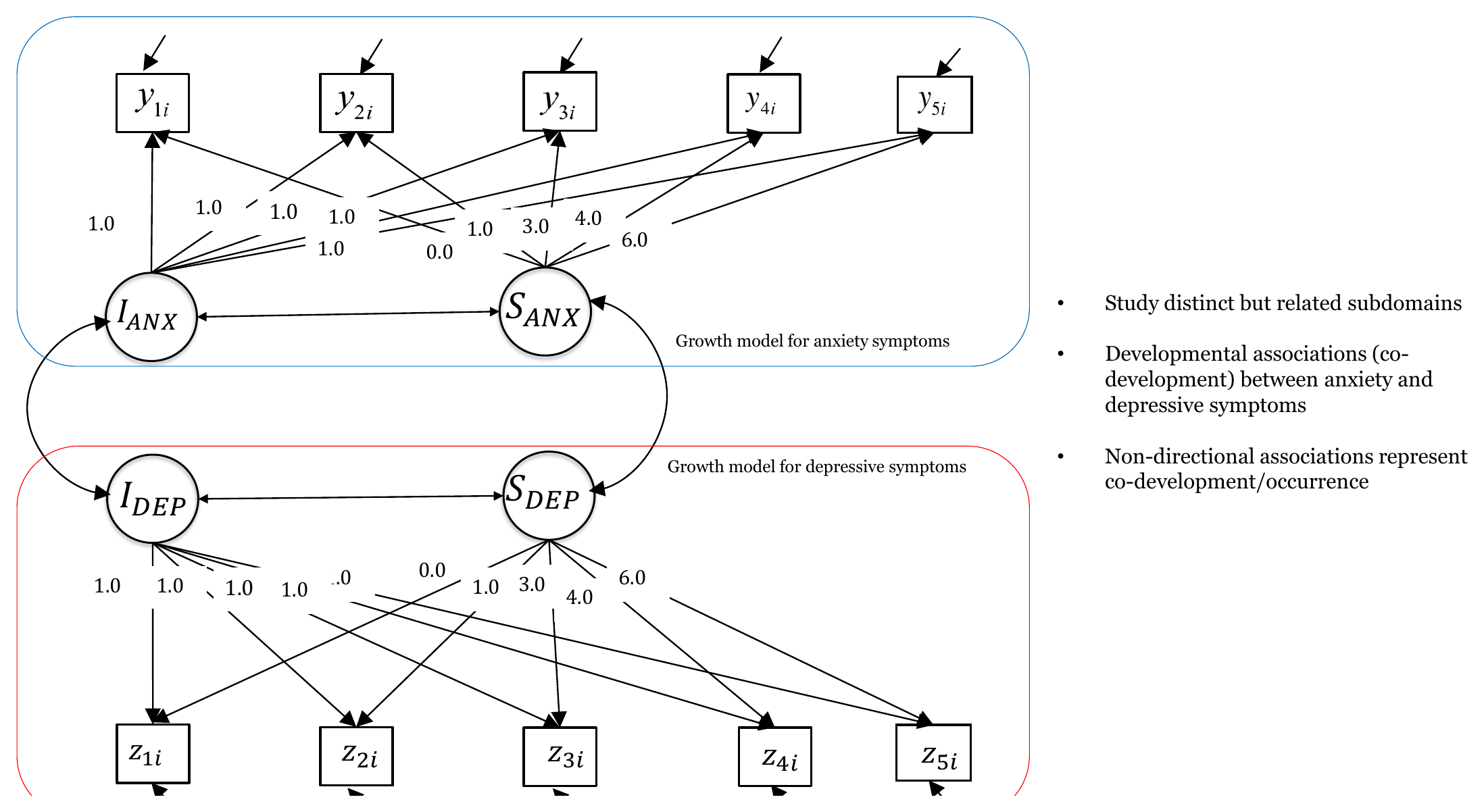{#fig-parallel-diagram fig-alt="Path diagram with growth factors for anxiety and depression, loadings 1 and 0, 1, 3, 4, 6, and double-headed arrows between the growth factors" width="90%"}### Understanding the outputThe model converges and uses `r lavInspect(fit_parallel, "nobs")` of the `r n_all` rows. @fig-parallel-results shows the workshop slide with the results. The slide reports Mplus estimates. The numbers in this chapter are from the R output above, and they agree with the slide to the reported precision.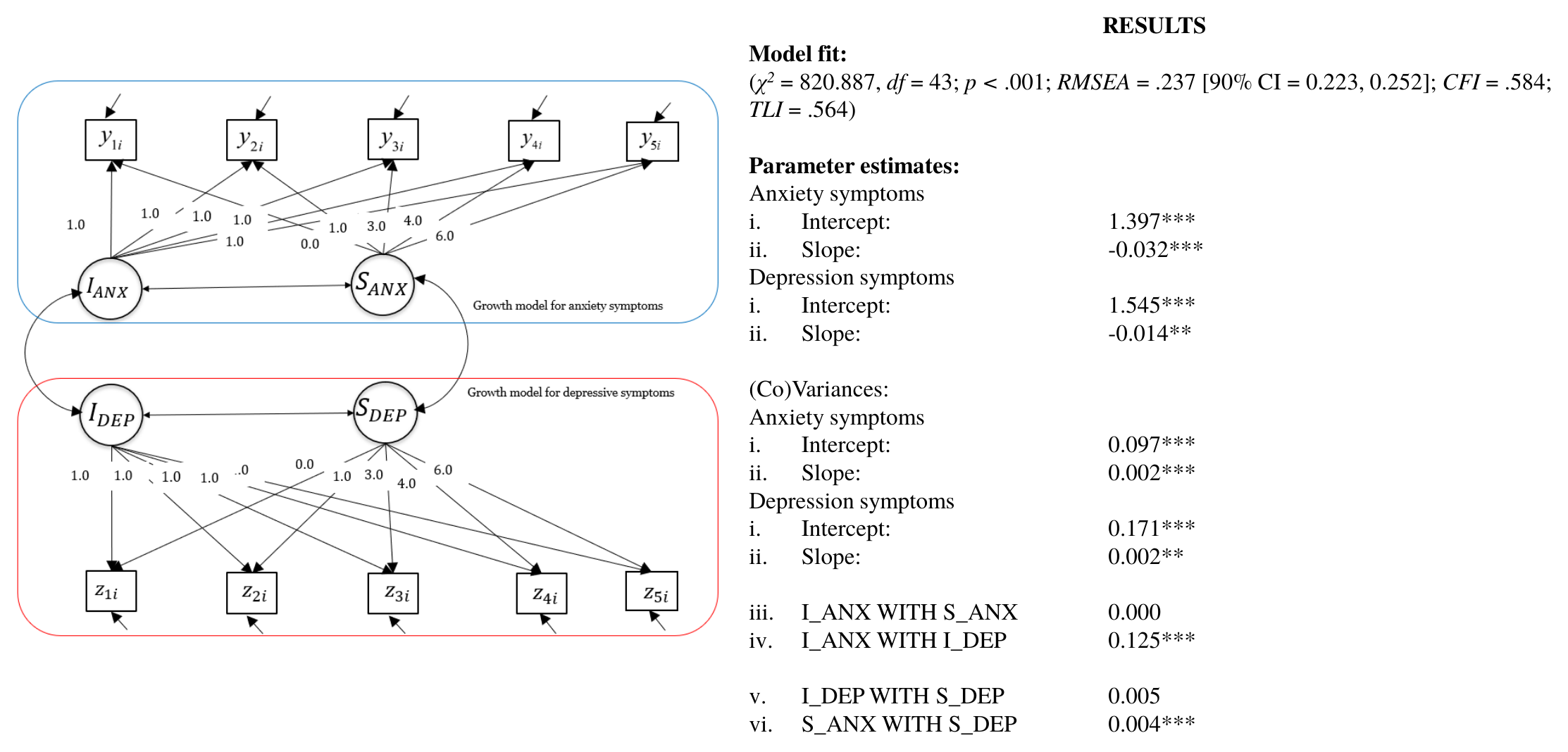{#fig-parallel-results fig-alt="Path diagram of the parallel growth model with model fit and parameter estimates for anxiety and depression" width="90%"}The fit is poor. We find $\chi^2(`r fitMeasures(fit_parallel, "df")`) = `r CH(fit_parallel)`$, CFI = `r FM(fit_parallel, "cfi")`, TLI = `r FM(fit_parallel, "tli")`, RMSEA = `r FM(fit_parallel, "rmsea")` (90% CI `r FM(fit_parallel, "rmsea.ci.lower")` to `r FM(fit_parallel, "rmsea.ci.upper")`) and SRMR = `r FM(fit_parallel, "srmr")`. These values are far from the usual reference values for an acceptable fit [@hu1999cutoff]. The model reproduces the covariances among the ten variables badly.The anxiety intercept is `r E(fit_parallel, "ia", "~1", "")` and the anxiety slope is `r E(fit_parallel, "sa", "~1", "")` (*p* `r PV(fit_parallel, "sa", "~1", "")`). The depression intercept is `r E(fit_parallel, "id", "~1", "")` and the depression slope is `r E(fit_parallel, "sd", "~1", "")` (*p* `r PV(fit_parallel, "sd", "~1", "")`). So the average level at the first wave is about `r fx(getp(fit_parallel, "ia", "~1", "")$est, 1)` for anxiety and `r fx(getp(fit_parallel, "id", "~1", "")$est, 1)` for depression, and both averages decrease slightly per year. Over the six years from the first to the fifth wave, the model implies an average change of `r f3(6 * getp(fit_parallel, "sa", "~1", "")$est)` for anxiety and `r f3(6 * getp(fit_parallel, "sd", "~1", "")$est)` for depression, on the scale of the scores.The variances of the growth factors are all different from zero according to the z tests. The variance of the intercept is `r E(fit_parallel, "ia", "~~", "ia")` for anxiety and `r E(fit_parallel, "id", "~~", "id")` for depression. The variance of the slope is only `r E(fit_parallel, "sa", "~~", "sa")` for anxiety and `r E(fit_parallel, "sd", "~~", "sd")` for depression. The slope variances are small in absolute terms, which is expected for a change per year.The covariances among the growth factors answer the questions of the chapter, but the lavaan warning below must be kept in mind. It shows that the covariance of the two slopes cannot be interpreted. The covariance between the two intercepts is `r E(fit_parallel, "ia", "~~", "id")` (SE = `r SE(fit_parallel, "ia", "~~", "id")`, z = `r ZV(fit_parallel, "ia", "~~", "id")`, *p* `r PV(fit_parallel, "ia", "~~", "id")`). The covariance between the two slopes is `r E(fit_parallel, "sa", "~~", "sd")` (z = `r ZV(fit_parallel, "sa", "~~", "sd")`, *p* `r PV(fit_parallel, "sa", "~~", "sd")`). Within the anxiety domain the covariance of intercept and slope is `r E(fit_parallel, "ia", "~~", "sa")` (*p* `r PV(fit_parallel, "ia", "~~", "sa")`), and within the depression domain it is `r E(fit_parallel, "id", "~~", "sd")` (*p* `r PV(fit_parallel, "id", "~~", "sd")`). The covariance of the two intercepts is positive, which means that participants who start higher on anxiety also start higher on depression.### The lavaan warninglavaan prints a warning for this model: the covariance matrix of the latent variables is not positive definite. This is the covariance matrix of the four growth factors. A covariance matrix is not positive definite when some combination of the variables has a negative variance, which cannot happen for real variables. The estimates are then not a possible set of variances and covariances.@tbl-latent-checks collects the checks for the three models. For the parallel growth model, the variances of the four growth factors are positive, but the correlation between the two slopes that the estimates imply is `r fx(rl(fit_parallel)["sa", "sd"], 2)`. A correlation cannot be larger than 1. The covariance of the two slopes (`r E(fit_parallel, "sa", "~~", "sd", 4)`) is larger than the product of the standard deviations of the slopes allows. The correlation between the two intercepts is `r fx(rl(fit_parallel)["ia", "id"], 2)`, which is close to the limit. The smallest eigenvalue of the covariance matrix of the growth factors is `r f5(min(eigen(lavInspect(fit_parallel, "cov.lv"))$values))`, and it is negative, which is how lavaan detects the problem.Notice that each slope has a variance close to zero, and that a covariance with a factor that hardly varies is difficult to estimate. The slope covariance in this model is large relative to these variances. Therefore the covariance of the two slopes in this model is not a result that we can interpret.## The model with autocorrelated residuals### Why we add autocorrelationsThe poor fit of the parallel growth model suggests that the residuals are not unrelated. A first candidate is the relation of a variable with itself over adjacent waves. After removing the person-specific line, a participant who scores above the line at one wave could still score above the line at the next wave. This is called an autocorrelated residual. The workshop slides draw these covariances as curved arrows between neighboring variables of a domain (@fig-autocor-diagram). The model does not say what the source of such a covariance is.### R implementationIn the workshop script this is model 10.2. Eight lines are added to the parallel growth model. The four lines for anxiety share the label `eqa` and the four lines for depression share the label `eqd`. Lines that share a label are held equal. Therefore the model has one autocorrelation for anxiety and one for depression, each assumed to be the same for all adjacent pairs of waves.```{r}#| label: autocor-modelparallelautocor <-' ia =~ 1*anx1 + 1*anx2 + 1*anx3 + 1*anx4 + 1*anx5 sa =~ 0*anx1 + 1*anx2 + 3*anx3 + 4*anx4 + 6*anx5 id =~ 1*dep1 + 1*dep2 + 1*dep3 + 1*dep4 + 1*dep5 sd =~ 0*dep1 + 1*dep2 + 3*dep3 + 4*dep4 + 6*dep5#Growth factor corelationsia ~~ id + sasd ~~ id + saia ~~ 0*sdid ~~ 0*sa#Autocorrelationsanx1 ~~ eqa*anx2anx2 ~~ eqa*anx3anx3 ~~ eqa*anx4anx4 ~~ eqa*anx5dep1 ~~ eqd*dep2dep2 ~~ eqd*dep3dep3 ~~ eqd*dep4dep4 ~~ eqd*dep5'fit_parallelautocor <-growth(parallelautocor, data = data)summary(fit_parallelautocor, fit.measures =TRUE)```The equality constraint is a simplification. The waves are one, two, one and two years apart, and the dependence between residuals of waves that are two years apart need not be the same as for waves that are one year apart. Holding the covariances equal keeps the model small.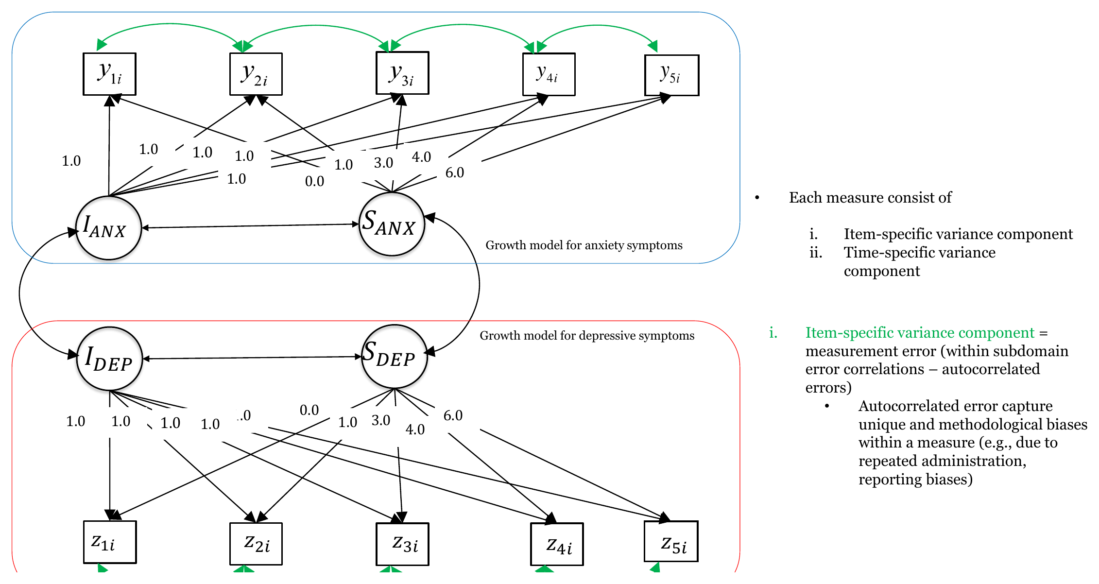{#fig-autocor-diagram fig-alt="Path diagram of the parallel growth model with green curved arrows between residuals of adjacent waves within anxiety and within depression" width="90%"}### Understanding the output@fig-autocor-results shows the slide with the results. It reports Mplus estimates, and the lower part of the slide is cropped. The chapter uses the R output.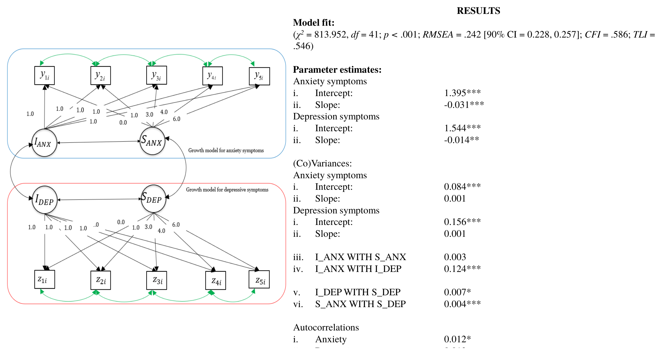{#fig-autocor-results fig-alt="Path diagram of the model with autocorrelated residuals with model fit and parameter estimates" width="90%"}The model uses the same `r lavInspect(fit_parallelautocor, "nobs")` participants. The fit is as poor as before: $\chi^2(`r fitMeasures(fit_parallelautocor, "df")`) = `r CH(fit_parallelautocor)`$, CFI = `r FM(fit_parallelautocor, "cfi")`, TLI = `r FM(fit_parallelautocor, "tli")`, RMSEA = `r FM(fit_parallelautocor, "rmsea")` (90% CI `r FM(fit_parallelautocor, "rmsea.ci.lower")` to `r FM(fit_parallelautocor, "rmsea.ci.upper")`) and SRMR = `r FM(fit_parallelautocor, "srmr")`. The model has two more parameters than the parallel growth model, so two degrees of freedom less.The autocorrelation for anxiety (`eqa`) is `r E(fit_parallelautocor, "anx1", "~~", "anx2")` (SE = `r SE(fit_parallelautocor, "anx1", "~~", "anx2")`, z = `r ZV(fit_parallelautocor, "anx1", "~~", "anx2")`, *p* `r PV(fit_parallelautocor, "anx1", "~~", "anx2")`). The autocorrelation for depression (`eqd`) is `r E(fit_parallelautocor, "dep1", "~~", "dep2")` (SE = `r SE(fit_parallelautocor, "dep1", "~~", "dep2")`, z = `r ZV(fit_parallelautocor, "dep1", "~~", "dep2")`, *p* `r PV(fit_parallelautocor, "dep1", "~~", "dep2")`). The two values are similar in size, but only the first is distinguishable from zero given its standard error. On the correlation scale, the residuals of adjacent waves correlate about `r fx(standardizedSolution(fit_parallelautocor) |> filter(lhs == "anx1", rhs == "anx2") |> pull(est.std), 2)` for anxiety and `r fx(standardizedSolution(fit_parallelautocor) |> filter(lhs == "dep1", rhs == "dep2") |> pull(est.std), 2)` for depression. These are small correlations.The growth factors change as well. The slope variances are `r E(fit_parallelautocor, "sa", "~~", "sa")` for anxiety (*p* `r PV(fit_parallelautocor, "sa", "~~", "sa")`) and `r E(fit_parallelautocor, "sd", "~~", "sd")` for depression (*p* `r PV(fit_parallelautocor, "sd", "~~", "sd")`). In the parallel growth model both slope variances were significant. Now neither is distinguishable from zero. Some of the variation that was assigned to the slopes in the parallel growth model may be wave-specific variation that is now taken by the residual covariances.The same warning appears again. The covariance matrix of the latent variables is not positive definite. The variances of the slopes are positive, but the estimated covariance between the two slopes (`r E(fit_parallelautocor, "sa", "~~", "sd")`) implies a correlation of `r fx(rl(fit_parallelautocor)["sa", "sd"], 2)`, and the correlation of the two intercepts is `r fx(rl(fit_parallelautocor)["ia", "id"], 2)`. Both are above 1 (see @tbl-latent-checks).### What changed compared with the parallel growth modelThe parallel growth model is the model with autocorrelated residuals in which the two autocorrelations are fixed at zero. So the two models are nested, and the likelihood ratio test applies. The change in fit is small. The chi-square decreases by `r f3(fitMeasures(fit_parallel, "chisq") - fitMeasures(fit_parallelautocor, "chisq"))` for two degrees of freedom. This suggests that carryover from wave to wave within a domain is a small part of what the first model misses.## The model with cross-domain residual covariances### Why we add cross-domain covariancesThe correlations in @tbl-cross-cor suggest another place to look. The two domains correlate strongly at the same wave and much less across different waves. The growth factors describe differences between persons that are stable over the waves. Because the slope variances are small, they mainly imply a covariance between an anxiety score and a depression score that is similar for any pair of waves. The data show a much higher covariance at the same wave. This is a covariance between the residuals of the two domains, specific to the wave. The workshop slides label it the time-specific component between the domains (@fig-cross-diagram).### R implementationIn the workshop script this is model 10.3. The five new lines connect the anxiety residual with the depression residual at the same wave, and they all share the label `eq`. The autocorrelations of the previous model are not part of this model.```{r}#| label: cross-modelparallelcross <-' ia =~ 1*anx1 + 1*anx2 + 1*anx3 + 1*anx4 + 1*anx5 sa =~ 0*anx1 + 1*anx2 + 3*anx3 + 4*anx4 + 6*anx5 id =~ 1*dep1 + 1*dep2 + 1*dep3 + 1*dep4 + 1*dep5 sd =~ 0*dep1 + 1*dep2 + 3*dep3 + 4*dep4 + 6*dep5#Growth factor corelationsia ~~ id + sasd ~~ id + saia ~~ 0*sdid ~~ 0*sa#Cross domain correlationsanx1 ~~ eq*dep1anx2 ~~ eq*dep2anx3 ~~ eq*dep3anx4 ~~ eq*dep4anx5 ~~ eq*dep5'fit_parallelcross <-growth(parallelcross, data = data)summary(fit_parallelcross, fit.measures =TRUE)```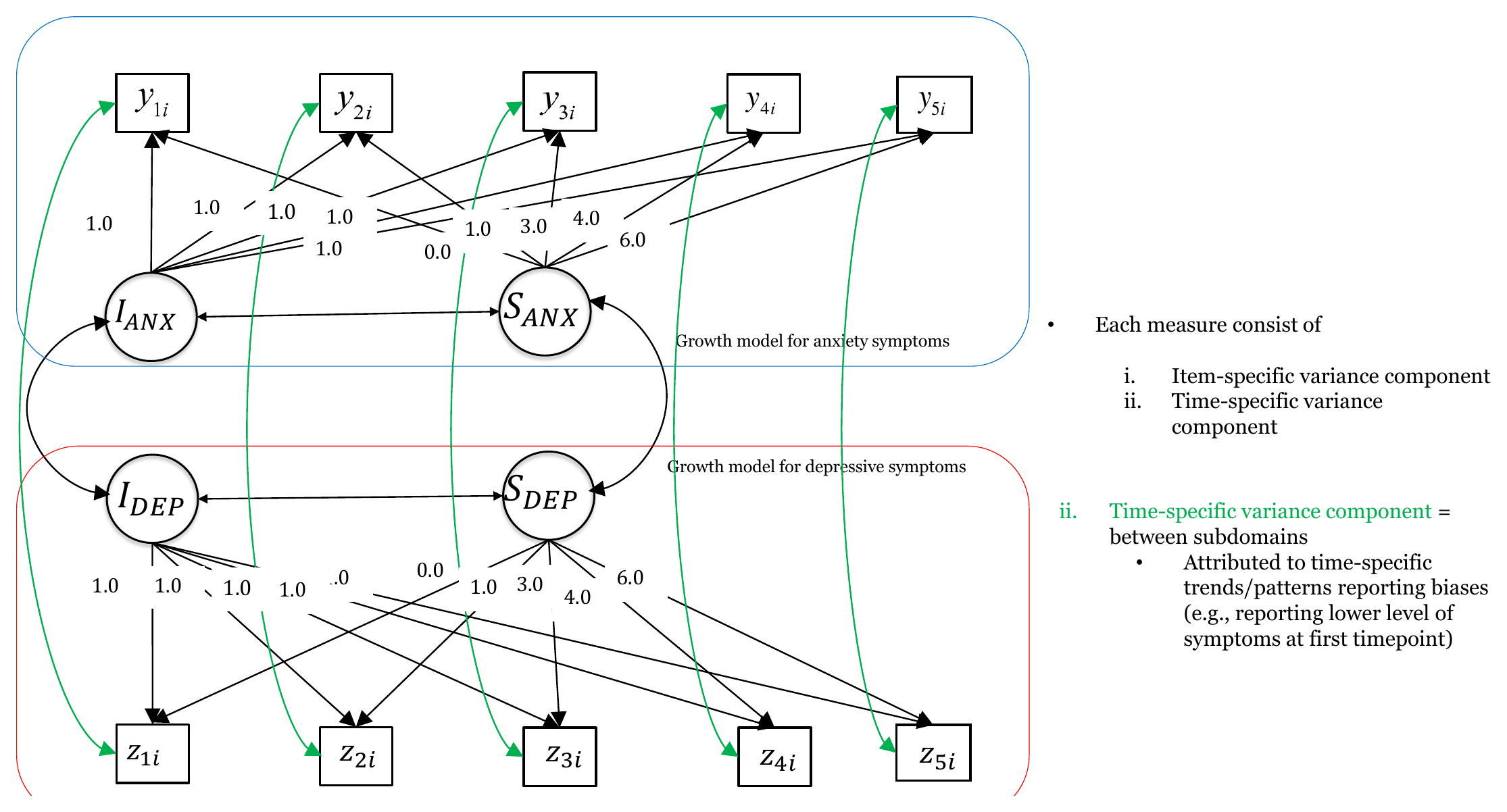{#fig-cross-diagram fig-alt="Path diagram of the parallel growth model with green curved arrows between the anxiety and depression residuals at each of the five waves" width="90%"}### Understanding the output@fig-cross-results shows the workshop slide with the results. It reports Mplus estimates, and the lower part of the slide is cropped, but the cross-domain covariance is visible. The chapter uses the R output.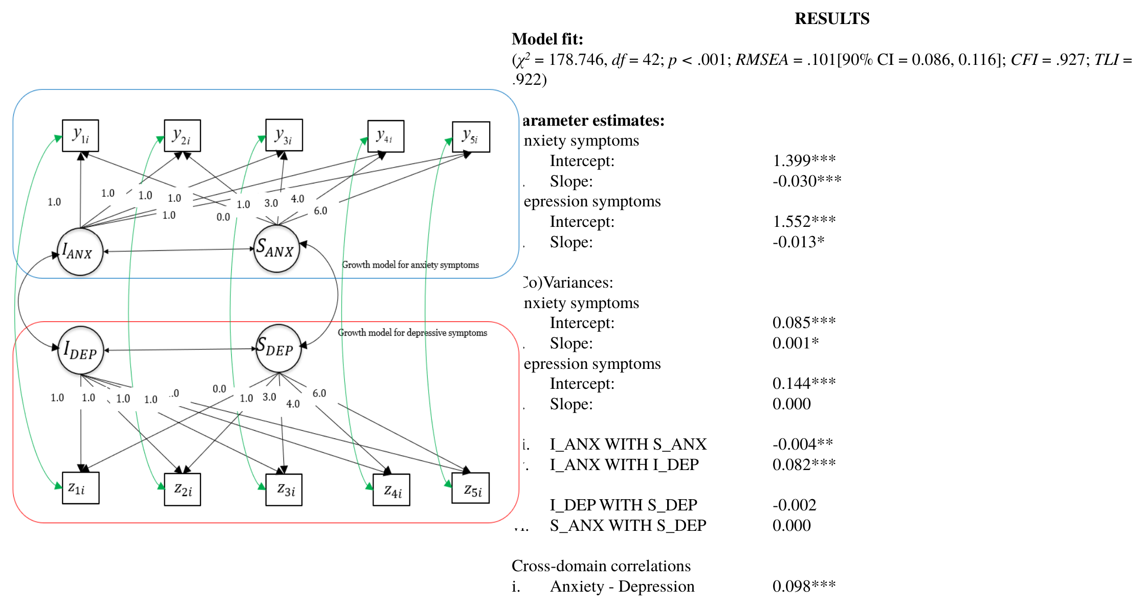{#fig-cross-results fig-alt="Path diagram of the model with cross-domain residual covariances with model fit and parameter estimates" width="90%"}```{r}#| label: std-cross#| include: falsesc <-standardizedSolution(fit_parallelcross)std_cross <-sapply(1:5, function(k) sc$est.std[sc$lhs ==paste0("anx", k) & sc$op =="~~"& sc$rhs ==paste0("dep", k)])```The model again uses `r lavInspect(fit_parallelcross, "nobs")` participants and has one parameter more than the parallel growth model. The fit improves a great deal: $\chi^2(`r fitMeasures(fit_parallelcross, "df")`) = `r CH(fit_parallelcross)`$, CFI = `r FM(fit_parallelcross, "cfi")`, TLI = `r FM(fit_parallelcross, "tli")`, RMSEA = `r FM(fit_parallelcross, "rmsea")` (90% CI `r FM(fit_parallelcross, "rmsea.ci.lower")` to `r FM(fit_parallelcross, "rmsea.ci.upper")`) and SRMR = `r FM(fit_parallelcross, "srmr")`. This is the best fit of the three models, but it is not a well fitting model by the usual reference values [@hu1999cutoff]. The CFI is below .95, and the RMSEA and the SRMR are above .08. The substantive reading below is therefore tentative.The cross-domain residual covariance (`eq`) is `r E(fit_parallelcross, "anx1", "~~", "dep1")` (SE = `r SE(fit_parallelcross, "anx1", "~~", "dep1")`, z = `r ZV(fit_parallelcross, "anx1", "~~", "dep1")`, *p* `r PV(fit_parallelcross, "anx1", "~~", "dep1")`). On the correlation scale this is `r fx(standardizedSolution(fit_parallelcross) |> filter(lhs == "anx1", rhs == "dep1") |> pull(est.std), 2)` at the first wave and `r fx(standardizedSolution(fit_parallelcross) |> filter(lhs == "anx5", rhs == "dep5") |> pull(est.std), 2)` at the fifth wave. This is a large amount of shared wave-specific variation. After removing the growth factors, the anxiety and the depression scores of the same wave still correlate between `r fx(min(std_cross), 2)` and `r fx(max(std_cross), 2)` across the five waves.The covariance is held equal across waves, but the residual variances differ between waves, so the standardized correlation differs too (`r fx(std_cross[3], 2)` at the third wave, against `r fx(std_cross[1], 2)` and `r fx(std_cross[5], 2)` at the first and the fifth). The equality constraint has not been tested here.The growth factors change as well.- The covariance of the two intercepts decreases from `r E(fit_parallel, "ia", "~~", "id")` to `r E(fit_parallelcross, "ia", "~~", "id")`, and it remains clearly positive (SE = `r SE(fit_parallelcross, "ia", "~~", "id")`, z = `r ZV(fit_parallelcross, "ia", "~~", "id")`, *p* `r PV(fit_parallelcross, "ia", "~~", "id")`). The correlation of the intercepts falls from `r fx(rl(fit_parallel)["ia", "id"], 2)` in the parallel growth model to about `r fx(rl(fit_parallelcross)["ia", "id"], 2)`.- The covariance of the two slopes is `r E(fit_parallelcross, "sa", "~~", "sd", 4)` (*p* `r PV(fit_parallelcross, "sa", "~~", "sd")`). In the two previous models it was `r E(fit_parallel, "sa", "~~", "sd")` (*p* `r PV(fit_parallel, "sa", "~~", "sd")`) and `r E(fit_parallelautocor, "sa", "~~", "sd")` (*p* `r PV(fit_parallelautocor, "sa", "~~", "sd")`). It involves the depression slope factor, whose variance is negative in this model, and it cannot be interpreted (see the warning below).- The covariance of intercept and slope in anxiety is now `r E(fit_parallelcross, "ia", "~~", "sa")` (*p* `r PV(fit_parallelcross, "ia", "~~", "sa")`). In depression it is `r E(fit_parallelcross, "id", "~~", "sd")` (*p* `r PV(fit_parallelcross, "id", "~~", "sd")`).- The average growth factors hardly change. The anxiety intercept and slope are `r E(fit_parallelcross, "ia", "~1", "")` and `r E(fit_parallelcross, "sa", "~1", "")`. The depression intercept and slope are `r E(fit_parallelcross, "id", "~1", "")` and `r E(fit_parallelcross, "sd", "~1", "")`.### The lavaan warningFor this model lavaan warns that some estimated latent variances are negative. The negative variance is that of the depression slope factor (`sd`). Its estimate is `r E(fit_parallelcross, "sd", "~~", "sd", 4)` (SE = `r SE(fit_parallelcross, "sd", "~~", "sd", 4)`, z = `r ZV(fit_parallelcross, "sd", "~~", "sd")`, *p* `r PV(fit_parallelcross, "sd", "~~", "sd")`). Negative variance estimates of this kind are discussed by @dillon1987offending. A variance cannot be negative, so the estimate has to be read as zero. The standard error is larger than the estimate, which means that the data are consistent with a variance of exactly zero. In this model, once the shared wave-specific variation has been taken out, there is no detectable variation between persons in the rate of change in depression. In the parallel growth model the variance of the depression slope is `r E(fit_parallel, "sd", "~~", "sd")` (*p* `r PV(fit_parallel, "sd", "~~", "sd")`), so the result depends on the model. The variance of the slope of anxiety is also small (`r E(fit_parallelcross, "sa", "~~", "sa")`, *p* `r PV(fit_parallelcross, "sa", "~~", "sa")`).This has consequences for the covariances of the depression slope. A correlation with a factor that has no variance is not defined. For this reason @tbl-latent-checks cannot report the correlation of the depression slope factor with the other growth factors for this model, and the covariances of `sd` in the output (with `id` and with `sa`) should not be interpreted.```{r}#| label: tbl-latent-checks#| tbl-cap: "Checks on the covariance matrix of the four growth factors in the three models. The correlations are computed from the estimated variances and covariances. A correlation is missing when a variance is negative."lc <-rbind(latent_check(fit_parallel), latent_check(fit_parallelautocor),latent_check(fit_parallelcross))rownames(lc) <-c("Parallel growth model", "Autocorrelated residuals","Cross-domain residual covariances")options(knitr.kable.NA ="not defined")lc[is.nan(lc)] <-NAknitr::kable(lc, digits =4)```::: {.callout-warning title="A covariance can be significant and still be impossible"}In the parallel growth model and in the model with autocorrelated residuals the covariance of the two slopes has a very small standard error, and it looks like the most precisely estimated result of the model. @tbl-latent-checks shows that it corresponds to a correlation above 1. This is not possible. The estimates reach this value because the slope variances are close to zero while the covariance is not. Check the implied correlations with `cov2cor(lavInspect(fit, "cov.lv"))` whenever lavaan reports a latent covariance matrix that is not positive definite, before interpreting covariances among growth factors.:::In such a case a researcher can fix the variance of the slope factor to zero, drop the slope factor of that domain, or use more data. We do not change the workshop syntax here.### What changed compared with the previous modelsThe only change from the parallel growth model is the five residual covariances held equal, which is one parameter. The change in fit is large, and it is a statement about the correspondence between the model and the data. The data contain a large covariance between the two domains at the same wave, and the first two models had no way to represent it. The growth factors may have absorbed it, which may be why the intercepts correlated almost perfectly and why the slope covariance was an impossible value. When the same-wave covariance is allowed, the growth factors take more modest values.## Comparing the three models@tbl-fit-compare puts the fit of the three models next to each other.```{r}#| label: tbl-fit-compare#| tbl-cap: "Fit of the three models, N = 321 (listwise deletion). AIC and BIC are smaller for models that fit better."fits <-list("Parallel growth model"= fit_parallel,"Autocorrelated residuals"= fit_parallelautocor,"Cross-domain residual covariances"= fit_parallelcross)cmp <-t(sapply(fits, function(f)c(ChiSq =fitMeasures(f, "chisq"), df =fitMeasures(f, "df"),CFI =fitMeasures(f, "cfi"), RMSEA =fitMeasures(f, "rmsea"),SRMR =fitMeasures(f, "srmr"), AIC =AIC(f), BIC =BIC(f))))colnames(cmp) <-c("Chi-square", "df", "CFI", "RMSEA", "SRMR", "AIC", "BIC")knitr::kable(cmp, digits =c(3, 0, 3, 3, 3, 3, 3))```The first two models are nested. The parallel growth model results from the model with autocorrelated residuals when `eqa` and `eqd` are fixed at zero. The chi-square difference test of the two [@bentler1980significance] is```{r}#| label: anova-12anova(fit_parallel, fit_parallelautocor)```The reduced model is rejected at the .05 level, so the model with the two autocorrelations fits better in the statistical sense. The difference is small, `r f3(fitMeasures(fit_parallel, "chisq") - fitMeasures(fit_parallelautocor, "chisq"))` for two degrees of freedom, and both models fit very poorly. The Akaike information criterion [AIC, @akaike1974new] prefers the model with autocorrelated residuals (`r f3(AIC(fit_parallelautocor))` against `r f3(AIC(fit_parallel))`), and the Bayesian information criterion [BIC, @schwarz1978estimating] prefers the parallel growth model (`r f3(BIC(fit_parallel))` against `r f3(BIC(fit_parallelautocor))`). Remember that models should be compared in substantive terms only if their fit is acceptable. A statistically significant difference between two models that both fit badly does not make the better one a good model. Also, the usual reference distribution of the test does not hold when a variance is estimated at or near the boundary of zero [@self1987asymptotic], which is the case here (see the warnings above), so the *p* value is approximate.::: {.callout-note title="Nested and non-nested models"}The parallel growth model is nested in each of the two other models, because it is obtained by fixing their added parameters at zero. So `anova(fit_parallel, fit_parallelcross)` is a valid likelihood ratio test, with a chi-square difference of `r f3(fitMeasures(fit_parallel, "chisq") - fitMeasures(fit_parallelcross, "chisq"))` for one degree of freedom. The model with autocorrelated residuals and the model with cross-domain residual covariances are not nested, because each has parameters that the other does not have. Their chi-square values cannot be tested against each other. Information criteria can be compared for non-nested models fitted to the same data, which is the case here.:::The model with cross-domain residual covariances has an AIC of `r f3(AIC(fit_parallelcross))` and a BIC of `r f3(BIC(fit_parallelcross))`. Both are lower than the values of the model with autocorrelated residuals, by `r f3(AIC(fit_parallelautocor) - AIC(fit_parallelcross))` (AIC) and `r f3(BIC(fit_parallelautocor) - BIC(fit_parallelcross))` (BIC), and this agrees with all fit indices in @tbl-fit-compare. The comparison with the second model is made with the information criteria alone. Both criteria and all fit indices put the model with cross-domain residual covariances first. The order of the two other models depends on the criterion.## Sensitivity to the missing data handlingThe models above are based on `r n_cc` of the `r n_all` rows. As a check, which is not part of the workshop, the three models were also fitted with full information maximum likelihood (FIML, see @sec-prelims). FIML was found to perform better than listwise deletion in the conditions examined by @enders2001relative.```{r}#| label: tbl-fiml#| tbl-cap: "Sensitivity analysis, not part of the workshop. Fit of the three models with listwise deletion and with FIML."dg <-read.csv("data/diag/diagnostics_summary.csv")dg <- dg[dg$label %in%c("010_1_parallel", "010_2_autocor", "010_3_cross"), ]tab_fiml <-data.frame(Model =c("Parallel growth model", "Autocorrelated residuals","Cross-domain residual covariances"),N_listwise = dg$n_listwise, CFI = dg$cfi, RMSEA = dg$rmsea,N_FIML = dg$n_fiml, CFI_FIML = dg$cfi_fiml, RMSEA_FIML = dg$rmsea_fiml,SRMR_FIML = dg$srmr_fiml)knitr::kable(tab_fiml, digits =3)``````{r}#| label: fiml-values#| include: falseest_all <-read.csv("data/diag/estimates_listwise_vs_fiml.csv")g <-function(label, lhs, op, rhs, col) { est_all[est_all$label == label & est_all$lhs == lhs & est_all$op == op & est_all$rhs == rhs, col][1]}cor_fiml <-function(label, a, b) {g(label, a, "~~", b, "est_fiml") /sqrt(g(label, a, "~~", a, "est_fiml") *g(label, b, "~~", b, "est_fiml"))}```The FIML models use N = `r dg$n_fiml[1]`. The pattern is the same as with listwise deletion. The first two models fit poorly (CFI `r fx(dg$cfi_fiml[1])` and `r fx(dg$cfi_fiml[2])`), and the model with cross-domain residual covariances fits better (CFI `r fx(dg$cfi_fiml[3])`, RMSEA `r fx(dg$rmsea_fiml[3])`, SRMR `r fx(dg$srmr_fiml[3])`). With the robust maximum likelihood estimator [@yuan2000three] and FIML, the CFI of the third model is `r fx(dg$cfi_mlr[3])`, which meets the usual cut-off of .95, and the RMSEA is `r fx(dg$rmsea_mlr[3])`. The RMSEA and the SRMR under FIML are still above .08 [@hu1999cutoff].The growth factor means hardly change. For example, the anxiety intercept in the model with cross-domain residual covariances is `r f3(g("010_3_cross", "ia", "~1", "", "est_lw"))` with listwise deletion and `r f3(g("010_3_cross", "ia", "~1", "", "est_fiml"))` with FIML. The variances are somewhat larger under FIML, for instance the variance of the anxiety intercept in this model is `r f3(g("010_3_cross", "ia", "~~", "ia", "est_lw"))` and `r f3(g("010_3_cross", "ia", "~~", "ia", "est_fiml"))`. The cross-domain residual covariance is `r f3(g("010_3_cross", "anx1", "~~", "dep1", "est_lw"))` and `r f3(g("010_3_cross", "anx1", "~~", "dep1", "est_fiml"))`. The variance of the depression slope in this model is `r f5(g("010_3_cross", "sd", "~~", "sd", "est_fiml"))` under FIML (SE = `r f5(g("010_3_cross", "sd", "~~", "sd", "se_fiml"))`) against `r f5(g("010_3_cross", "sd", "~~", "sd", "est_lw"))` with listwise deletion. Under FIML the estimate is positive, but it is not distinguishable from zero. So the factor has little variance to estimate in both analyses.The correlation of the two intercepts is `r fx(cor_fiml("010_1_parallel", "ia", "id"), 2)` in the parallel growth model and `r fx(cor_fiml("010_3_cross", "ia", "id"), 2)` in the model with cross-domain residual covariances under FIML. This is the same pattern as with listwise deletion, with a value at or just above the limit of 1 in the first model.## A check on the two constraints at zeroThe two covariances that are fixed at zero, `ia ~~ 0*sd` and `id ~~ 0*sa`, are part of the three workshop models. Nothing in the data requires them, so we can check what happens when they are estimated. The code below is an addition to the workshop. It is the model with cross-domain residual covariances, with the two covariances freed.```{r}#| label: free-constraints# Addition, not part of the workshop: the two covariances fixed at zero are freedparallelcross_free <-' ia =~ 1*anx1 + 1*anx2 + 1*anx3 + 1*anx4 + 1*anx5 sa =~ 0*anx1 + 1*anx2 + 3*anx3 + 4*anx4 + 6*anx5 id =~ 1*dep1 + 1*dep2 + 1*dep3 + 1*dep4 + 1*dep5 sd =~ 0*dep1 + 1*dep2 + 3*dep3 + 4*dep4 + 6*dep5ia ~~ id + sa + sdsd ~~ id + said ~~ saanx1 ~~ eq*dep1anx2 ~~ eq*dep2anx3 ~~ eq*dep3anx4 ~~ eq*dep4anx5 ~~ eq*dep5'fit_parallelcross_free <-growth(parallelcross_free, data = data)anova(fit_parallelcross, fit_parallelcross_free)parameterEstimates(fit_parallelcross_free) |>filter(op =="~~", lhs %in%c("ia", "sa", "id", "sd"), rhs %in%c("ia", "sa", "id", "sd")) |>select(lhs, rhs, est, se, z, pvalue)```lavaan gives no warning for this model, and all four growth factor variances are positive. The smallest eigenvalue of the covariance matrix of the growth factors is `r f5(min(eigen(lavInspect(fit_parallelcross_free, "cov.lv"))$values))`, so the matrix is positive definite. The model fits better than the model of the workshop: $\chi^2(`r fitMeasures(fit_parallelcross_free, "df")`) = `r CH(fit_parallelcross_free)`$, CFI = `r FM(fit_parallelcross_free, "cfi")`, RMSEA = `r FM(fit_parallelcross_free, "rmsea")` and SRMR = `r FM(fit_parallelcross_free, "srmr")`. The chi-square difference with the model of the workshop [@bentler1980significance] is `r f3(fitMeasures(fit_parallelcross, "chisq") - fitMeasures(fit_parallelcross_free, "chisq"))` for two degrees of freedom. The two freed covariances are `r E(fit_parallelcross_free, "ia", "~~", "sd")` (anxiety intercept with depression slope) and `r E(fit_parallelcross_free, "sa", "~~", "id")` (depression intercept with anxiety slope), and the output shows that both are distinguishable from zero.So the two constraints at zero are not harmless in this dataset. They may be part of the reason why a negative slope variance appears in the model with cross-domain residual covariances. We should not make much of the particular values of these covariances. They involve slope factors with variances of `r E(fit_parallelcross_free, "sa", "~~", "sa")` and `r E(fit_parallelcross_free, "sd", "~~", "sd")` (*p* `r PV(fit_parallelcross_free, "sd", "~~", "sd")` for the depression slope factor, which is positive here), and such correlations are unstable. The fit, even with the covariances freed, is still not good by the usual reference values. Thus, a warning about a latent variance can come from a constraint we imposed.## What these models answer and what they cannot tellThe parallel growth model answers the question whether two growth processes are associated across persons. In this dataset the initial levels of anxiety and depression are positively related in all three models, and the association is strong. The correlation of the intercepts is `r fx(rl(fit_parallel)["ia", "id"], 2)` and `r fx(rl(fit_parallelautocor)["ia", "id"], 2)` in the first two models (the second is above 1) and about `r fx(rl(fit_parallelcross)["ia", "id"], 2)` in the model with cross-domain residual covariances, which fits best of the three but is still not a well fitting model. The association between the two rates of change cannot be read from these models. In the first two it corresponds to a correlation above 1, and in the third the depression slope factor has a negative variance. With the two covariances freed the implied correlation of the slopes is `r fx(rl(fit_parallelcross_free)["sa", "sd"], 2)`, but the slope variances are very small, so this value is unstable. The data do not allow a strong claim about the co-development of the rates of change.The models do not tell why the two domains covary at the same wave. The covariance of the residuals in the third model absorbs everything that is shared by the anxiety and the depression score of a wave and is not carried by the growth factors. The data do not tell us what this shared variation is. The models also do not give a direction. A parallel growth model does not describe an influence of one process on the other, and both processes cover the same period. A model in which one process comes before the other in time is the topic of @sec-sequential.## Researcher's perspectiveThe models use `r n_cc` of `r n_all` rows. A model with two outcomes needs complete data on both, so the loss of cases is larger than in a single-outcome model. Report the N used, and consider FIML as a check.Residual covariances can change the growth factors considerably, as the change of the slope variances and of the slope covariance shows. Models that differ only in the residual structure can give different answers to the same question about the growth factors. It is therefore useful to report more than one structure when the choice is not clear, and to say which one is used for the substantive reading.The autocorrelations are held equal across waves that are one and two years apart, and the cross-domain covariance is held equal across five waves. These constraints are common, and they can be relaxed and tested if the sample is large enough. The constraints at zero between the growth factors of different domains define the model in the workshop, and they can be freed.::: {.callout-tip title="What to report"}Report the N used and the method for missing data, the fit indices of each model including those that fit badly, any lavaan warning and what it refers to, the implied correlations among the growth factors if a warning about the latent covariance matrix appears, and which residual structure the substantive reading is based on. State that the improvement in fit from the residual covariances is a statement about how well the model reproduces the data.:::