Code
data <- data %>%
  rename("dep6"  = "dep1",
         "dep7"  = "dep2",
         "dep8"  = "dep3",
         "dep9"  = "dep4",
"dep10" = "dep5")In Chapter 9 we fitted growth models for two processes, anxiety symptoms and depression symptoms, measured at the same five waves. The question there was whether the two processes go together. In this chapter we ask a question about order. Does a process that comes first in one domain go together with a process that comes later in another domain? Models that address this question are called sequential (or sequentially contingent) growth models.
A parallel growth model describes two processes that run side by side over the same stretch of time. It says nothing about which process comes first. A sequential design is different. An earlier process in one domain is followed by a later process in another domain, and the two are measured at different times. Take for example a first domain measured at five waves and a second domain measured at five later waves. The growth factors of the first process (initial level and rate of change) can then be related to the growth factors of the second process, and the model respects the fact that the second process happens after the first.
The dataset in this compendium does not contain a sequential design. In the workshop, the same five anxiety measurements and the same five depression measurements (waves 1 to 5) are relabeled as ten consecutive time points. Anxiety is called T1 to T5 and depression is called T6 to T10, with depression time scores 0, 1, 2, 3 and 4. Nothing was measured after wave 5. The purpose is to show how the syntax of a sequential model is built. The estimates of the model below are not to be interpreted substantively.
Three features of the syntax matter. The variables of the later domain are renamed so that they occupy later time points, the time scores of the later domain restart at zero, and the growth factors of the two domains are related through cross-domain covariances, here ia ~~ id and sa ~~ sd. These features carry over to real data.
The model is two linear growth models, one after the other. The first is the anxiety model with its intercept factor ia and slope factor sa. The second is the depression model with its intercept factor id and slope factor sd. Each model has its own time scores. For the second model, time starts again at zero at its own first wave, so that id is the expected level at the first wave of the second process and sd is the rate of change per unit of its own time. The coding of time decides what the intercept means (Biesanz et al., 2004).
The two models are then joined at the level of the growth factors. The covariance ia ~~ id tells us whether people with a higher initial level of anxiety also have a higher initial level of depression. The covariance sa ~~ sd tells us whether people who change faster in anxiety also change faster in depression. Remember that a covariance has no direction. If the theory says that the earlier process should predict the later one, the covariances can be replaced by regressions. The workshop syntax carries a comment to this effect, but the model fitted here uses covariances only.
The dataset contains anxiety symptoms (anx1 to anx5) and depression symptoms (dep1 to dep5) for the same participants at the same five waves. As in earlier chapters, the anxiety slope uses the time scores 0, 1, 3, 4 and 6, which follow the spacing of the waves (1, 2, 1 and 2 years).
To build a model with ten consecutive time points, the depression variables are renamed. The variable dep1 becomes dep6, dep2 becomes dep7, and so on up to dep5, which becomes dep10. The depression slope then uses the time scores 0, 1, 2, 3 and 4. Notice two things about this setup. The numbers in the data are unchanged, since only the names of the columns differ. And the equal spacing of the depression time scores does not describe the real spacing of these measurements, which were taken at the same uneven intervals as the anxiety measurements. In the parallel model of Chapter 9 the depression scores were therefore given the time scores 0, 1, 3, 4 and 6.
A real sequential design would look different. The anxiety measurements could come from one period, for example waves 1 to 5, and the depression measurements from a later period, for example waves 6 to 10, collected after the first set. The time scores of depression would restart at zero at wave 6 and would follow the real spacing of waves 6 to 10. In that case the intercept id would be the initial level of depression after the anxiety process has run its course. This is not the situation here, because id is simply the expected depression score at wave 1 under a new name.
For person \(i\), the anxiety scores at time points \(t = 1, \dots, 5\) and the depression scores at time points \(t = 6, \dots, 10\) follow two linear growth models.
\[ \text{anx}_{ti} = \eta_{0i}^{(a)} + \lambda_t^{(a)} \, \eta_{1i}^{(a)} + \epsilon_{ti}, \qquad \lambda^{(a)} = (0, 1, 3, 4, 6) \]
\[ \text{dep}_{ti} = \eta_{0i}^{(d)} + \lambda_t^{(d)} \, \eta_{1i}^{(d)} + \epsilon_{ti}, \qquad \lambda^{(d)} = (0, 1, 2, 3, 4) \]
In the syntax, \(\eta_0^{(a)}\) is ia, \(\eta_1^{(a)}\) is sa, \(\eta_0^{(d)}\) is id and \(\eta_1^{(d)}\) is sd. The four growth factors have means and a covariance matrix \(\Psi\). With the factors ordered as ia, sa, id, sd, the matrix has this pattern.
\[ \Psi = \begin{pmatrix} \psi_{ia} & & & \\ \psi_{ia,sa} & \psi_{sa} & & \\ \psi_{ia,id} & 0 & \psi_{id} & \\ 0 & \psi_{sa,sd} & \psi_{id,sd} & \psi_{sd} \end{pmatrix} \]
The four variances and four covariances are freely estimated. The two covariances that mix an intercept of one domain with the slope of the other domain (ia with sd and sa with id) are fixed to zero. The ten residual variances are freely estimated, and the residuals are not correlated. Together with the four growth factor means this gives 10 + 4 + 4 + 4 = 22 parameters.
We start from the same setup as in the other chapters.
The function growth() reads a loading such as 1*dep6 and looks for a column called dep6. It does not know that this column holds the first depression scores. Therefore, the renaming is done with dplyr::rename() before the model is written.
data <- data %>%
rename("dep6" = "dep1",
"dep7" = "dep2",
"dep8" = "dep3",
"dep9" = "dep4",
"dep10" = "dep5")After a rename, look at names(data) before fitting. If a loading refers to a column that does not exist, lavaan stops with an error. If it refers to the wrong column, there is no error at all and the model is simply wrong.
The model is fitted with growth() (Rosseel, 2012). It has two growth models and the covariances between their growth factors. The time scores of sa and sd are different, because the second set restarts at zero.
sequential <- ' ia =~ 1*anx1 + 1*anx2 + 1*anx3 + 1*anx4 + 1*anx5
                sa =~ 0*anx1 + 1*anx2 + 3*anx3 + 4*anx4 + 6*anx5
                id =~ 1*dep6 + 1*dep7 + 1*dep8 + 1*dep9 + 1*dep10
                sd =~ 0*dep6 + 1*dep7 + 2*dep8 + 3*dep9 + 4*dep10

#Growth factor corelations
ia ~~ sa
id ~~ sd
ia ~~ 0*sd
id ~~ 0*sa

#Correlate growth factors across domain (may use regressions depending on theory?)
ia ~~ id
sa ~~ sd
'

fit_sequential <- growth(sequential, data = data)
summary(fit_sequential, fit.measures = TRUE)
lavaan 0.6.17 ended normally after 94 iterations
Estimator ML
Optimization method NLMINB
Number of model parameters 22
Used Total
Number of observations 321 442
Model Test User Model:
Test statistic 825.260
Degrees of freedom 43
P-value (Chi-square) 0.000
Model Test Baseline Model:
Test statistic 1912.994
Degrees of freedom 45
P-value 0.000
User Model versus Baseline Model:
Comparative Fit Index (CFI) 0.581
Tucker-Lewis Index (TLI) 0.562
Loglikelihood and Information Criteria:
Loglikelihood user model (H0) -1713.264
Loglikelihood unrestricted model (H1) -1300.634
Akaike (AIC) 3470.529
Bayesian (BIC) 3553.501
Sample-size adjusted Bayesian (SABIC) 3483.720
Root Mean Square Error of Approximation:
RMSEA 0.238
90 Percent confidence interval - lower 0.224
90 Percent confidence interval - upper 0.252
P-value H_0: RMSEA <= 0.050 0.000
P-value H_0: RMSEA >= 0.080 1.000
Standardized Root Mean Square Residual:
SRMR 0.357
Parameter Estimates:
Standard errors Standard
Information Expected
Information saturated (h1) model Structured
Latent Variables:
Estimate Std.Err z-value P(>|z|)
ia =~
anx1 1.000
anx2 1.000
anx3 1.000
anx4 1.000
anx5 1.000
sa =~
anx1 0.000
anx2 1.000
anx3 3.000
anx4 4.000
anx5 6.000
id =~
dep6 1.000
dep7 1.000
dep8 1.000
dep9 1.000
dep10 1.000
sd =~
dep6 0.000
dep7 1.000
dep8 2.000
dep9 3.000
dep10 4.000
Covariances:
Estimate Std.Err z-value P(>|z|)
ia ~~
sa 0.000 0.002 0.038 0.970
id ~~
sd 0.007 0.004 1.987 0.047
ia ~~
sd 0.000
sa ~~
id 0.000
ia ~~
id 0.124 0.012 10.339 0.000
sa ~~
sd 0.005 0.001 9.077 0.000
Intercepts:
Estimate Std.Err z-value P(>|z|)
ia 1.397 0.021 65.125 0.000
sa -0.032 0.004 -7.806 0.000
id 1.546 0.028 56.233 0.000
sd -0.021 0.008 -2.778 0.005
Variances:
Estimate Std.Err z-value P(>|z|)
.anx1 0.081 0.010 8.466 0.000
.anx2 0.123 0.011 11.102 0.000
.anx3 0.148 0.012 11.892 0.000
.anx4 0.102 0.009 11.541 0.000
.anx5 0.066 0.008 7.894 0.000
.dep6 0.102 0.013 7.726 0.000
.dep7 0.153 0.014 10.946 0.000
.dep8 0.239 0.020 11.852 0.000
.dep9 0.181 0.016 11.558 0.000
.dep10 0.158 0.016 9.777 0.000
ia 0.097 0.012 8.387 0.000
sa 0.002 0.000 3.989 0.000
id 0.171 0.020 8.648 0.000
sd 0.005 0.002 2.749 0.006The model was fitted to 321 of the 442 participants (listwise deletion, see Chapter 1). The chi-square statistic is 825.260 with 43 degrees of freedom, CFI is .581, TLI is .562, RMSEA is .238 (90% CI .224 to .252) and SRMR is .357. By the usual cut-offs (Hu & Bentler, 1999) this is a poor fit on every index. The data to model correspondence is weak, and the model is not one that we would take forward to a substantive interpretation.
As in Chapter 9, lavaan prints a warning that the covariance matrix of the latent variables is not positive definite. The estimated covariance matrix of ia, sa, id and sd is therefore not a valid covariance matrix, and its smallest eigenvalue is -0.003, which is below zero (lavInspect(fit_sequential, "cov.lv")). The implied correlation between sa and sd is 1.761. A correlation above 1 is impossible, so this is an inadmissible solution. The variance of sa is very small (0.002) and the covariance of sa with sd is large relative to it. The options for a researcher are the ones given in Chapter 9. We leave the workshop syntax unchanged here.
Figure 10.1 shows the diagram and the results from the workshop slides. The slide reports Mplus estimates. The numbers in this chapter are the ones from the R output, and they agree with the slide to three decimals for the fit statistics, the growth factor means, the variances and the covariances. The one visible difference concerns the covariance of id with sd, which the slide shows without a significance marker. The R output gives p = .047, which is borderline.
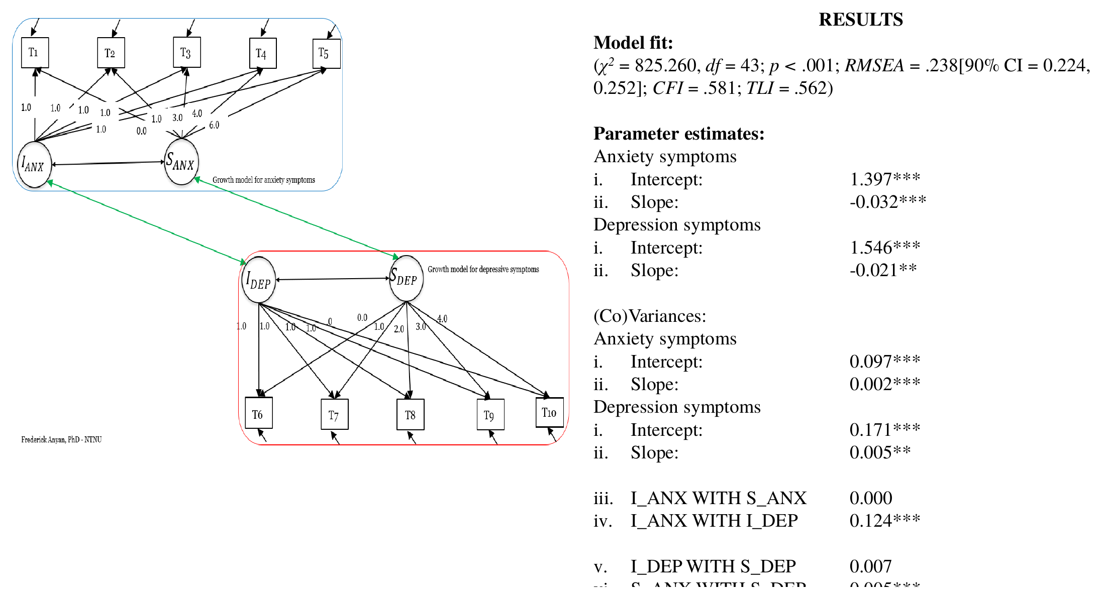
Growth factor means. The anxiety intercept is 1.397 and the anxiety slope is -0.032. The depression intercept is 1.546 and the depression slope is -0.021. All four means differ from zero (p < .05).
Growth factor variances. The variances are 0.097 for ia, 0.002 for sa, 0.171 for id and 0.005 for sd. The slope variances are close to zero, and that of sa is the source of the warning above.
Covariances. Within the anxiety domain, the covariance of ia with sa is 0.000 (p = .970). Within the depression domain, the covariance of id with sd is 0.007 (p = .047). The two cross-domain covariances are 0.124 for ia with id and 0.005 for sa with sd. The two covariances fixed to zero (ia with sd and sa with id) have no standard errors, as in the output.
Residual variances. They range from 0.066 to 0.148 for the anxiety variables and from 0.102 to 0.239 for the depression variables. They are freely estimated at each wave.
Given the fit and the warning, we describe the numbers as properties of this relabeled model and not as findings. The means suggest that both domains have a slightly negative slope on average, with an average slope of -0.032 per year for anxiety and -0.021 per time unit of the restarted scale for depression. The covariance of the two intercepts is positive and clearly different from zero, and the implied correlation is very high (0.962). People with a higher anxiety score at the first wave tend to have a higher depression score at the first wave. This is a statement about two sets of scores taken at the same waves, since id is the depression level at wave 1.
For this reason the cross-domain covariances of this model cannot be read as an earlier process going together with a later one. The anxiety and depression scores that the model places at different time points were collected at the same waves. The data contain no information on order. The covariance of sa with sd corresponds to a correlation above 1 and is not interpretable. This is the same problem as for the slopes in the parallel model of Chapter 9.
The sequential model of this chapter and the parallel model of Chapter 9 use the same four growth factors. They differ in the renaming of the depression variables, in the time scores of depression (0, 1, 3, 4 and 6 in the parallel model and 0, 1, 2, 3 and 4 here) and in the way the covariances are written. The parallel syntax has the lines ia ~~ id + sa, sd ~~ id + sa, ia ~~ 0*sd and id ~~ 0*sa. The sequential syntax separates the within-domain covariances (ia ~~ sa, id ~~ sd, ia ~~ 0*sd, id ~~ 0*sa) from the cross-domain ones (ia ~~ id, sa ~~ sd) and comments on them. Both specifications leave the same four covariances free and fix the same two to zero, so the covariance structure is identical. To compare the two models in numbers, we fit the parallel model again with the original variable names.
data_orig <- read.csv("data/data.csv", fileEncoding = "UTF-8-BOM")

parallel <- ' ia =~ 1*anx1 + 1*anx2 + 1*anx3 + 1*anx4 + 1*anx5
              sa =~ 0*anx1 + 1*anx2 + 3*anx3 + 4*anx4 + 6*anx5
              id =~ 1*dep1 + 1*dep2 + 1*dep3 + 1*dep4 + 1*dep5
              sd =~ 0*dep1 + 1*dep2 + 3*dep3 + 4*dep4 + 6*dep5
ia ~~ id + sa
sd ~~ id + sa
ia ~~ 0*sd
id ~~ 0*sa
'
fit_parallel <- growth(parallel, data = data_orig)fp <- fitMeasures(fit_parallel)
pp <- parameterEstimates(fit_parallel)
pk <- function(lhs, op, rhs) pp[pp$lhs == lhs & pp$op == op & pp$rhs == rhs, "est"]
sk <- function(lhs, op, rhs) pick(lhs, op, rhs)
cmp <- data.frame(
Quantity = c("CFI", "RMSEA", "SRMR",
"Mean of ia", "Mean of sa", "Mean of id", "Mean of sd",
"Variance of sd", "Covariance ia with id",
"Covariance sa with sd", "Covariance id with sd"),
Sequential = c(fm["cfi"], fm["rmsea"], fm["srmr"],
sk("ia", "~1", ""), sk("sa", "~1", ""), sk("id", "~1", ""), sk("sd", "~1", ""),
sk("sd", "~~", "sd"), sk("ia", "~~", "id"),
sk("sa", "~~", "sd"), sk("id", "~~", "sd")),
Parallel = c(fp["cfi"], fp["rmsea"], fp["srmr"],
pk("ia", "~1", ""), pk("sa", "~1", ""), pk("id", "~1", ""), pk("sd", "~1", ""),
pk("sd", "~~", "sd"), pk("ia", "~~", "id"),
pk("sa", "~~", "sd"), pk("id", "~~", "sd"))
)
knitr::kable(cmp, digits = 3, row.names = FALSE, align = "lrr")| Quantity | Sequential | Parallel |
|---|---|---|
| CFI | 0.581 | 0.584 |
| RMSEA | 0.238 | 0.237 |
| SRMR | 0.357 | 0.357 |
| Mean of ia | 1.397 | 1.397 |
| Mean of sa | -0.032 | -0.032 |
| Mean of id | 1.546 | 1.545 |
| Mean of sd | -0.021 | -0.014 |
| Variance of sd | 0.005 | 0.002 |
| Covariance ia with id | 0.124 | 0.125 |
| Covariance sa with sd | 0.005 | 0.004 |
| Covariance id with sd | 0.007 | 0.005 |
Table 10.1 shows that the two models fit the data about equally badly (CFI .581 and .584). The anxiety part is nearly the same, as it should be. The differences are in the depression slope. The mean of sd is -0.021 in the sequential model and -0.014 in the parallel model. Their ratio is 1.46. The two sets of time scores are not proportional, but the last score is 4 in one and 6 in the other, and the ratio is roughly 6 / 4 = 1.5. The same scores spread over a shorter time metric give a steeper slope per unit. Time scores define the unit in which the slope is expressed, and changing them changes the slope and its variance even when the data and the covariance structure are the same.
When the second process starts at zero, its time scores must still reflect the real time between its own waves. Equal steps such as 0, 1, 2, 3 and 4 are only correct if the measurements are equally spaced. In this chapter they are not correct for the data, and we use them to show the syntax. Never copy the time scores of one domain to another because the number of waves is the same. See Chapter 1 for the role of time scores.
With data from a real sequential design, the model can answer whether the initial level and the rate of change of an earlier process are related to the initial level and the rate of change of a later process in a different domain. The covariances describe the association between growth factors across the two periods. Replacing them with regressions would add a direction to the association, depending on the theory.
It cannot tell us why the processes are related. The data are observational, and the model does not support causal statements. In addition, the model of this chapter has no information on order, as explained above. It cannot tell us anything about sequence for these data, and its fit and its warning do not allow a substantive reading.
Before fitting a sequential model, check whether the design is really sequential, which means that the second process is measured after the first. If both domains are measured at the same waves, the parallel model is the one to use. The time scores of each domain must follow the real spacing of its own waves. Whether the cross-domain links should be covariances or regressions depends on the theory.
The workshop code uses listwise deletion, so only 321 of the 442 participants contribute (see Chapter 1 for the sensitivity check with full information maximum likelihood). A near-zero variance, as seen here, is a reason to check the data and the model before reporting anything. If you fit a sequential model to your own data, report the fit, the warnings, the time scores of each domain and the way the covariances were specified. For the model in this chapter, report that it was fitted to relabeled data as a demonstration of the syntax.